1.5) Tabular Data with pandas

pandas is the workhorse for labelled, tabular data: the Series (a labelled 1D array) and the DataFrame (named columns sharing an index). This notebook loads a small table of daily station observations — air temperature and river discharge at two stations, with realistic sensor gaps — and works through reading, selecting, time-indexing, rolling windows, grouping, and joining. The running theme is treating missing data as physical information the sensor recorded, rather than smoothing it away — exactly the choice the generated-code bug at the end gets wrong.

Figure 1:The pandas logo, designed by Marc Garcia for the project and taken from Wikimedia Commons; pandas itself is BSD-3-Clause licensed.

1.5.1 Series and DataFrame¶

A Series pairs values with an index; a DataFrame is a collection of columns sharing one index. Each column has its own dtype.

import numpy as np
import pandas as pd

# a Series: values with a labelled index
temps = pd.Series([18.2, 17.5, 19.1],
                  index=["2024-06-01", "2024-06-02", "2024-06-03"],
                  name="temp_celsius")
print(temps)

# a DataFrame: named columns sharing an index
df = pd.DataFrame({"temp_celsius": [18.2, 17.5, 19.1],
                   "discharge_m3s": [48.0, 51.2, 47.5]})
print(df)
print(df.dtypes.to_dict())

2024-06-01    18.2
2024-06-02    17.5
2024-06-03    19.1
Name: temp_celsius, dtype: float64
   temp_celsius  discharge_m3s
0          18.2           48.0
1          17.5           51.2
2          19.1           47.5
{'temp_celsius': dtype('float64'), 'discharge_m3s': dtype('float64')}

1.5.2 Reading a CSV Robustly¶

read_csv infers types, but for analysis you should be explicit: parse date columns to datetime64, and pin the dtype of key columns. First we generate an example file; csv writing is covered near the end.

# --- generate an example data file (uses tools covered later; just setup here) ---
from pathlib import Path

Path("_files").mkdir(exist_ok=True)

rng = np.random.default_rng(0)
dates = pd.date_range("2024-06-01", periods=45, freq="D")
parts = []
for name, base_temp, base_q in [("BAS", 18.0, 50.0), ("LUG", 21.0, 30.0)]:
    parts.append(pd.DataFrame({
        "date": dates,
        "station": name,
        "temp_celsius": (base_temp + rng.normal(0, 1.5, 45)).round(1),
        "discharge_m3s": (base_q + rng.normal(0, 5, 45)).round(1),
    }))
raw = pd.concat(parts, ignore_index=True)
raw.loc[[3, 4, 50], "temp_celsius"] = np.nan       # simulate sensor gaps
raw.to_csv("_files/station_observations.csv", index=False)
print("wrote station_observations.csv with", len(raw), "rows")

wrote station_observations.csv with 90 rows

obs = pd.read_csv(
    "_files/station_observations.csv",
    parse_dates=["date"],            # -> datetime64, not object strings
    dtype={"station": "string"},     # pin the key column's type
)
print(obs.dtypes.to_dict())
print(obs.head())

{'date': dtype('<M8[us]'), 'station': <StringDtype(na_value=<NA>)>, 'temp_celsius': dtype('float64'), 'discharge_m3s': dtype('float64')}
        date station  temp_celsius  discharge_m3s
0 2024-06-01     BAS          18.2           48.4
1 2024-06-02     BAS          17.8           57.3
2 2024-06-03     BAS          19.0           59.8
3 2024-06-04     BAS           NaN           59.0
4 2024-06-05     BAS           NaN           56.6

1.5.3 Selecting: .loc, .iloc, and Boolean Masks¶

.loc selects by label, .iloc by integer position, and a boolean mask filters rows by condition. Combine several conditions with & (and) and | (or) — not Python’s and/or from subchapter 1.2, which do not work element-wise on a Series — and wrap each condition in its own parentheses, since &/| bind more tightly than comparisons like == and >, so omitting them changes what gets evaluated.

# boolean indexing: warm days at Lugano
warm_lug = obs[(obs["station"] == "LUG") & (obs["temp_celsius"] > 22.0)]
print(warm_lug[["date", "temp_celsius"]].head())

# .iloc by position, .loc by label
print(obs.iloc[0].to_dict())          # first row, by position
print(obs.loc[0, "station"])          # one cell, by label

         date  temp_celsius
46 2024-06-02          23.4
56 2024-06-12          22.5
59 2024-06-15          22.3
71 2024-06-27          23.1
72 2024-06-28          22.1
{'date': Timestamp('2024-06-01 00:00:00'), 'station': 'BAS', 'temp_celsius': 18.2, 'discharge_m3s': 48.4}
BAS

1.5.4 Updating and Transforming Values¶

A column is created or overwritten by assignment, applied to every row at once. A boolean mask combined with .loc updates only the matching rows, leaving the rest untouched.

# a new column, computed for every row in one vectorised expression
obs["temp_fahrenheit"] = obs["temp_celsius"] * 9 / 5 + 32

# update only the matching rows, in place
obs.loc[obs["discharge_m3s"] > 55.0, "flow_flag"] = "high_flow"

print(obs[["station", "temp_celsius", "temp_fahrenheit", "flow_flag"]].head(3))

  station  temp_celsius  temp_fahrenheit  flow_flag
0     BAS          18.2            64.76        NaN
1     BAS          17.8            64.04  high_flow
2     BAS          19.0            66.20  high_flow

1.5.5 A datetime Index: resample and Rolling Windows¶

Setting a datetime index unlocks time-aware operations. resample re-bins to a coarser period; rolling computes a moving window.

# index one station by date
bas = obs[obs["station"] == "BAS"].set_index("date").sort_index()

print("monthly mean °C:", bas["temp_celsius"].resample("MS").mean().round(2).tolist())
# rolling on the gap-free discharge: the first 6 are NaN while the window fills
print("7-day rolling mean discharge (m3 s-1):")
print(bas["discharge_m3s"].rolling(window=7).mean().round(2).head(10).tolist())

monthly mean °C: [17.82, 18.39]
7-day rolling mean discharge (m3 s-1):
[nan, nan, nan, nan, nan, nan, 53.84, 54.07, 53.5, 51.19]

1.5.6 groupby: Split, Apply, Combine¶

groupby splits rows by a key, applies an aggregation to each group, and combines the results.

summary = obs.groupby("station").agg(
    mean_temp=("temp_celsius", "mean"),     # mean skips NaN
    max_discharge=("discharge_m3s", "max"),
    n_obs=("temp_celsius", "size"),         # size counts every row, NaN included
)
print(summary.round(2))

         mean_temp  max_discharge  n_obs
station                                 
BAS          18.02           60.0     45
LUG          20.88           39.1     45

nunique counts how many distinct values a column holds; idxmax (or idxmin) returns the label of the row holding the maximum (minimum) value — useful directly on a groupby result like summary above.

print("distinct stations:", obs["station"].nunique())
print("station with the warmest mean temperature:", summary["mean_temp"].idxmax())

distinct stations: 2
station with the warmest mean temperature: LUG

1.5.7 Quick Plots with .plot()¶

Series and DataFrames carry a .plot() method that wraps matplotlib: it reads the index for the x-axis and the column names for the legend, so a first look needs no fig, ax boilerplate. Pass kind= to choose the plot type, and ax= to draw into axes you already created — return to the explicit figure/axes model from subchapter 1.4 whenever a plot needs more control than this gives you. For right-skewed data — many small values and a few very large ones — pass logy=True to put the count axis on a log scale, so a long tail does not crush everything else into one corner.

import matplotlib.pyplot as plt

fig, ax = plt.subplots(figsize=(6, 3))
bas["temp_celsius"].plot(ax=ax, color="tab:red")
ax.set_ylabel("temperature (°C)")
ax.set_title("Basel, daily mean temperature")
plt.show()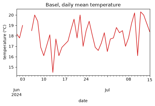

kind="bar" turns a grouped summary into a labelled bar chart in one line, reusing summary from the groupby above.

fig, ax = plt.subplots(figsize=(5, 3))
summary["mean_temp"].plot(ax=ax, kind="bar", color="tab:blue")
ax.set_ylabel("mean temperature (°C)")
ax.set_xlabel("station")
plt.show()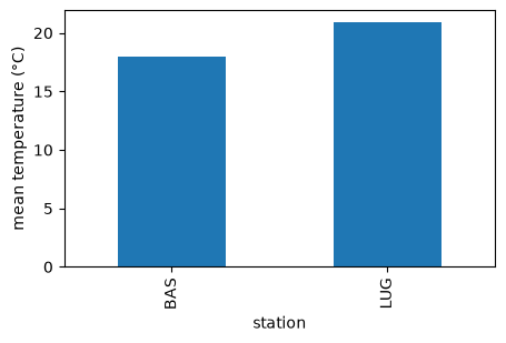

Many environmental quantities are right-skewed: most values sit near a typical range, with a long tail of rare, much larger ones. A linear count axis buries that tail near zero; passing logy=True spreads it out so both the common and the rare values are visible in the same plot.

# right-skewed data: a few very large values dominate a linear count axis
skewed = pd.Series(np.exp(rng.normal(3.0, 1.0, 500)))

fig, axes = plt.subplots(1, 2, figsize=(9, 3))
skewed.plot(ax=axes[0], kind="hist", color="tab:gray")
axes[0].set_title("linear count axis")
skewed.plot(ax=axes[1], kind="hist", color="tab:gray", logy=True)
axes[1].set_title("logy=True")
plt.tight_layout()
plt.show()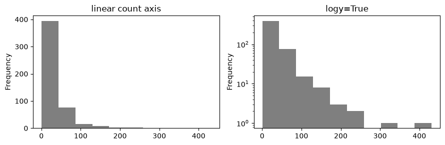

1.5.8 Missing Data as Physical Information¶

When a sensor stops reporting, the record should show that gap, not invent a reading. pandas marks missing values as NaN, detects them with isna, and its reductions skip them by default. How you fill a gap is a modelling choice: ffill carries the last value forward (sensible for slowly varying state), interpolate draws a straight line between neighbours.

# missing values per column — temp_celsius's gaps are genuine sensor dropouts;
# flow_flag's are a construction artifact of the .loc assignment above, which only
# wrote a string on high-flow rows and left every other row as NaN by default
print(obs.isna().sum().to_dict())

# two fills with different physical meaning
bas_temp = obs.loc[obs["station"] == "BAS", "temp_celsius"].reset_index(drop=True)
print("with gaps:  ", bas_temp.head(6).tolist())
print("ffill:      ", bas_temp.ffill().head(6).tolist())               # carry forward
print("interpolate:", bas_temp.interpolate().round(2).head(6).tolist())  # linear

{'date': 0, 'station': 0, 'temp_celsius': 3, 'discharge_m3s': 0, 'temp_fahrenheit': 3, 'flow_flag': 79}
with gaps:   [18.2, 17.8, 19.0, nan, nan, 18.5]
ffill:       [18.2, 17.8, 19.0, 19.0, 19.0, 18.5]
interpolate: [18.2, 17.8, 19.0, 18.83, 18.67, 18.5]

1.5.9 Combining Tables: merge and concat¶

merge joins tables on a shared key (a database-style join); concat stacks tables along an axis.

# join station metadata onto the observations
metadata = pd.DataFrame({
    "station": pd.array(["BAS", "LUG"], dtype="string"),
    "name": ["Basel-Binningen", "Lugano"],
    "elevation_m": [316, 273],
})
merged = obs.merge(metadata, on="station", how="left")
print(merged[["date", "station", "name", "elevation_m", "temp_celsius"]].head(3))

        date station             name  elevation_m  temp_celsius
0 2024-06-01     BAS  Basel-Binningen          316          18.2
1 2024-06-02     BAS  Basel-Binningen          316          17.8
2 2024-06-03     BAS  Basel-Binningen          316          19.0

Solution

lug = obs[obs["station"] == "LUG"].set_index("date").sort_index()
roll = lug["discharge_m3s"].rolling(window=7).mean()
print(round(roll.iloc[-1], 1))

1.5.10 Writing Outputs¶

Save results to disk with a pathlib path, which keeps the code OS-independent.

from pathlib import Path

out_path = Path("_files/station_summary.csv")
summary.to_csv(out_path)
print("wrote", out_path.name, "-", out_path.stat().st_size, "bytes")

wrote station_summary.csv - 99 bytes

When generated code lies: filling gaps with zero¶

Asked to “clean and average” a column with gaps, an assistant fills the missing values with zero and then takes the mean. The code runs, but zero is a valid temperature, so the gaps become spurious cold readings that drag the mean down.

def mean_temperature(df):
    # fill missing values, then average (as an assistant returned it)
    clean = df["temp_celsius"].fillna(0)
    return clean.mean()

bas_obs = obs[obs["station"] == "BAS"]
print("buggy mean:  ", round(mean_temperature(bas_obs), 2))
print("correct mean:", round(bas_obs["temp_celsius"].mean(), 2))   # skips NaN
print("gaps filled with 0 °C:", int(bas_obs["temp_celsius"].isna().sum()))

buggy mean:   17.22
correct mean: 18.02
gaps filled with 0 °C: 2

def mean_temperature(df):
    # reductions skip NaN already; interpolate only if a gap-free series is needed
    return df["temp_celsius"].mean()

print("fixed mean:", round(mean_temperature(bas_obs), 2))

fixed mean: 18.02

Going deeper: time zones

A naive timestamp has no zone; localize it, then convert.

idx = pd.date_range("2024-06-01", periods=3, freq="h")
aware = idx.tz_localize("UTC")          # attach UTC
local = aware.tz_convert("Europe/Zurich")   # convert to local clock time

Store and compute in UTC; convert to local time only for display.

Going deeper: multi-index

A hierarchical index lets one frame hold several grouping levels.

multi = obs.set_index(["station", "date"]).sort_index()
print(multi.loc["BAS"].head())      # select an outer level

groupby often produces a multi-index automatically when you group by more than one key.

Going deeper: apply

apply runs an arbitrary function per group or per row when no built-in aggregation fits.

spread = obs.groupby("station")["temp_celsius"].apply(lambda s: s.max() - s.min())

Prefer vectorised built-ins (mean, sum, agg) where they exist; apply is slower and should be the fallback, not the default.

Going deeper: Polars as a fast alternative

polars is a newer dataframe library with a lazy, multi-threaded engine that is often much faster on large data, with a more explicit expression API.

import polars as pl
df = pl.read_csv("_files/station_observations.csv")
df.group_by("station").agg(pl.col("temp_celsius").mean())

The concepts transfer directly from pandas; the syntax differs. It is shown for reference and not run here.

Summary¶

Concept	Rule to remember
Series and DataFrame	A Series is a labelled 1D array; a DataFrame is named columns sharing one index.
Reading	Be explicit: `parse_dates` for time columns, `dtype` for key columns.
Selecting	`.loc` by label, `.iloc` by position, boolean masks to filter.
Time	A datetime index is what enables `resample` and `rolling`.
Deriving	Assign to a column, or to a masked `.loc` selection — no loop needed.
Grouping and joining	`groupby` is split-apply-combine; `merge` joins on a key, `concat` stacks.
Missing data	Missing is not zero: detect with `isna`, and fill only as a deliberate physical choice.
The zero trap	`fillna(0)` silently biases every statistic whenever zero is itself a valid value.

Resources¶

Python for Data Analysis, 3rd ed. — Getting Started with pandas — McKinney; Series/DataFrame mechanics, selection, and the data-cleaning chapter that follows it.
pandas — Getting started — the official task-oriented tutorials for reading, selecting, grouping, and combining data.