

A Python for loop over a million temperature readings runs a million separate additions, each paying the interpreter’s overhead; numpy replaces the loop with one array operation that runs in compiled code, often one to two orders of magnitude faster, and reads closer to the mathematical statement of the problem. That combination — speed and a notation that matches the science — is why numpy underlies the rest of the scientific Python stack, from pandas to scikit-learn to xarray. This notebook works with one running example, a small two-dimensional temperature field on a latitude–longitude grid, to cover array creation, dtype and shape, indexing and masking, vectorised math and broadcasting, reductions, and the handling of missing data — the same topics numpy’s own beginner documentation covers, worth a look for a second pass at these ideas. It closes with a generated-code bug that silently truncates results because of a dtype mistake.

Figure 1:The NumPy logo, from the project’s own press kit, made available for use in course materials.
You already know a container for a sequence of numbers: the list. An ndarray differs in
three ways that matter for scientific work.
list | ndarray | |
|---|---|---|
| Dimensions | one (nested lists to fake more) | any number, as a real shape |
| Contents | anything, mixed | one dtype for every element |
| Arithmetic | * repeats, + joins | element-wise maths |
| Speed | a Python loop per element | one compiled loop over the whole block |
The single dtype is what buys the speed: because every element has the same type and size, numpy stores them in one contiguous block of memory and hands the loop to compiled code.
import numpy as np

py_list = [1, 2, 3, 4]
arr = np.array([1, 2, 3, 4])

print(py_list * 2)     # [1, 2, 3, 4, 1, 2, 3, 4] — the list is repeated
print(arr * 2)         # [2 4 6 8] — every element is doubled

# a list can hold mixed types; an array cannot
print(type(1).__name__, type("two").__name__, type(3.0).__name__)   # int str float
print(np.array([1, 2, 3]).dtype)                                    # int64 — one type for all
[1, 2, 3, 4, 1, 2, 3, 4]
[2 4 6 8]
int str float
int64
1.3.1 Creating arrays
An array is created from data — a nested list — or from a constructor. Every array carries a shape (its size along each axis) and an ndim (the number of axes).
import numpy as np

# a 2D field: 4 latitudes (rows) x 6 longitudes (cols), daily mean temp (°C)
temp_celsius = np.array([
    [ 5.2,  4.8,  6.1,  3.9,  2.7,  4.4],
    [ 1.3,  0.5, -0.8, -1.2,  0.9,  2.1],
    [-2.6, -3.1, -1.9,  0.2, -0.5,  1.1],
    [ 6.4,  7.0,  5.5,  8.1,  4.2,  5.8],
])

print(temp_celsius)
print("shape:", temp_celsius.shape, "| ndim:", temp_celsius.ndim)
[[ 5.2 4.8 6.1 3.9 2.7 4.4]
[ 1.3 0.5 -0.8 -1.2 0.9 2.1]
[-2.6 -3.1 -1.9 0.2 -0.5 1.1]
[ 6.4 7. 5.5 8.1 4.2 5.8]]
shape: (4, 6) | ndim: 2
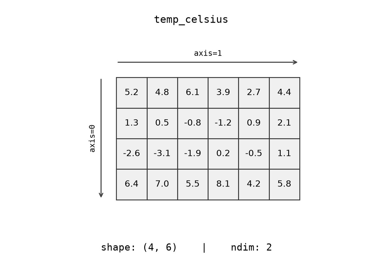
Figure 2:temp_celsius as a grid of 4 rows by 6 columns: shape is the size along each axis, ndim is the number of axes.
1.3.2 Other ways to create arrays
Beyond a literal, numpy provides constructors for the patterns you need most often.
print(np.zeros((2, 3)))          # all zeros, given shape
print(np.ones(4))                # all ones
print(np.full((2, 2), 7.0))      # filled with a constant
print(np.arange(0, 10, 2))       # evenly spaced by step: [0 2 4 6 8]
print(np.linspace(0.0, 1.0, 5))  # n evenly spaced points: [0. 0.25 0.5 0.75 1. ]
print(np.random.random(3))       # 3 random floats in [0, 1)
[[0. 0. 0.]
[0. 0. 0.]]
[1. 1. 1. 1.]
[[7. 7.]
[7. 7.]]
[0 2 4 6 8]
[0. 0.25 0.5 0.75 1. ]
[0.40166345 0.14912346 0.76739579]
Going deeper: dtype and precision
Every array also has a dtype — the element type — which fixes both its behaviour and its memory use. float64 (double precision) is the default; float32 halves the memory at the cost of precision.
temp32 = temp_celsius.astype(np.float32)
print(temp_celsius.dtype, temp_celsius.nbytes, "bytes")   # float64, 192 bytes
print(temp32.dtype, temp32.nbytes, "bytes")               # float32, 96 bytes

# float32 is coarser: the rounding error in 0.1 + 0.2 disappears
print(np.float64(0.1) + np.float64(0.2))   # 0.30000000000000004
print(np.float32(0.1) + np.float32(0.2))   # 0.3
Watch the dtype when preallocating output arrays with np.zeros_like: it silently copies the input’s dtype, so an integer input produces an integer output even when the result should be fractional.
Coordinates often come as two 1D axes, but a field defined on the grid needs a value at every
(row, column) pair. meshgrid expands the two axes into two 2D arrays of matching shape — one
holding the longitude of each cell, the other its latitude. You will use these constantly when
plotting fields in the next subchapter.
lon = np.linspace(6.0, 9.0, 6)     # 6 longitudes
lat = np.linspace(46.0, 47.5, 4)   # 4 latitudes

lon2d, lat2d = np.meshgrid(lon, lat)
print(lon2d.shape, lat2d.shape)    # (4, 6) (4, 6) — one value per grid cell
print(lon2d)
(4, 6) (4, 6)
[[6. 6.6 7.2 7.8 8.4 9. ]
[6. 6.6 7.2 7.8 8.4 9. ]
[6. 6.6 7.2 7.8 8.4 9. ]
[6. 6.6 7.2 7.8 8.4 9. ]]
1.3.3 Indexing, slicing, and boolean masking
Indexing uses [row, col]; slicing selects sub-blocks; negative indices count from the end. A boolean mask is a same-shaped array of True/False that selects the matching elements. Basic slicing (with :) returns a view, not a copy: it shares memory with the original array, so assigning into a slice also changes the array it was sliced from. Call .copy() on the slice when you need an independent array that you can change without touching the original.
print(temp_celsius[0, 0])      # one element
print(temp_celsius[0, :])      # first row, all longitudes
print(temp_celsius[:, -1])     # last column, all latitudes
print(temp_celsius[1:3, 2:4])  # a 2x2 sub-block

# a boolean mask and what it selects
freezing = temp_celsius < 0.0
print("n freezing cells:", int(freezing.sum()))    # True counts as 1
print("freezing values:", temp_celsius[freezing])  # 1D of matches
5.2
[5.2 4.8 6.1 3.9 2.7 4.4]
[4.4 2.1 1.1 5.8]
[[-0.8 -1.2]
[-1.9 0.2]]
n freezing cells: 6
freezing values: [-0.8 -1.2 -2.6 -3.1 -1.9 -0.5]
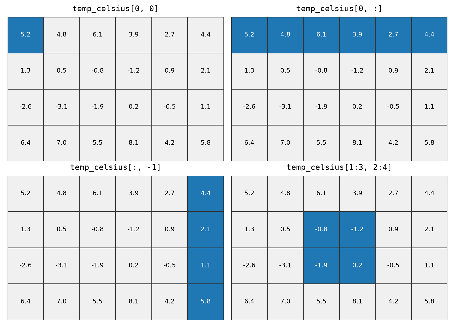
Figure 3:Four ways to select from temp_celsius: a single element, a full row, a full column, and a 2x2 sub-block.
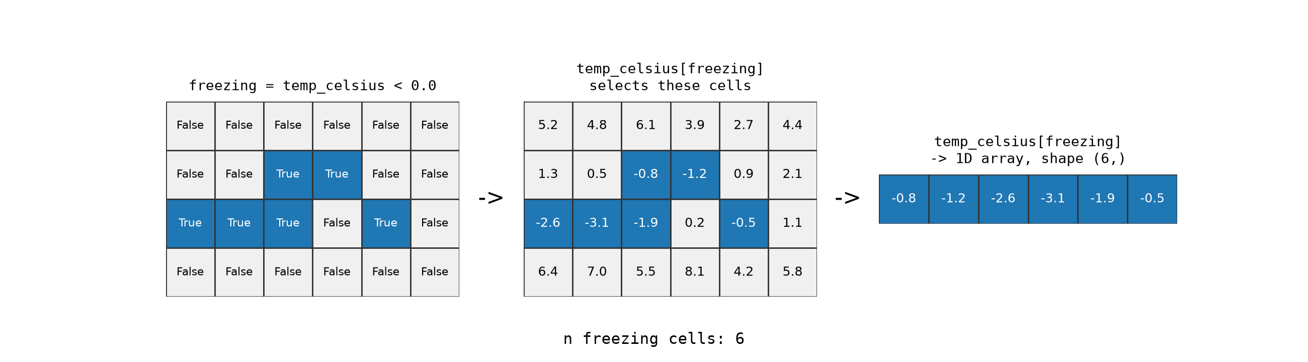
Figure 4:temp_celsius < 0.0 produces a same-shaped array of True/False; indexing with it, temp_celsius[freezing], pulls out the matching cells as a flat 1D array — not a row or a column, since the selected cells no longer form a rectangle.
Going deeper: memory layout, views, and strides
An array is a flat block of memory plus a shape and strides (the byte step along each axis). A slice is a view because it reuses the same block with a different starting point and different strides, so nothing has to be copied. C-order (row-major, the default) and Fortran-order (column-major) change which axis is contiguous and therefore which traversals are fastest.
a = np.arange(12).reshape(3, 4)
print(a.strides)          # bytes to step along (rows, cols)
b = a[:, 1]               # a view, not a copy
b[0] = 999                # this also changes a[0, 1]
1.3.4 Vectorised math and broadcasting
A single expression applies element-wise across an array. Broadcasting lets arrays of different but compatible shapes combine: a length-4 column vector can be stretched across all 6 longitudes.
# vectorised: no python loop
temp_kelvin = temp_celsius + 273.15
print(temp_kelvin)  # shape (4,6)
[[278.35 277.95 279.25 277.05 275.85 277.55]
[274.45 273.65 272.35 271.95 274.05 275.25]
[270.55 270.05 271.25 273.35 272.65 274.25]
[279.55 280.15 278.65 281.25 277.35 278.95]]
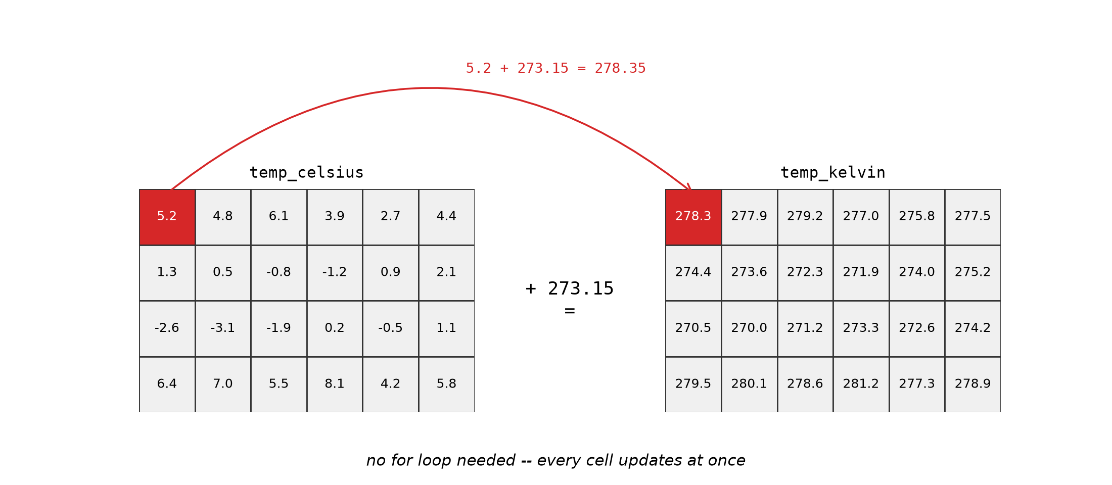
Figure 5:temp_celsius + 273.15 updates every cell in one expression — no for loop needed.
Broadcasting aligns shapes from the last axis backwards. Our field is (4, 6) and the latitude gradient is (4,) — numpy tries to match the 4 against the 6, fails, and raises an error. We have to say explicitly that the gradient varies along the rows, by giving it a second axis of length 1.
Indexing with None inserts a new axis at that position, turning a (4,) vector into a (4, 1) column. np.newaxis is the same thing spelled out, and you will see both.
lat_gradient_celsius = np.array([0.0, -1.5, -3.0, -4.5])   # colder toward the north

print(lat_gradient_celsius.shape)                  # (4,)   — a flat vector
print(lat_gradient_celsius[:, None].shape)         # (4, 1) — now a column
print(lat_gradient_celsius[:, np.newaxis].shape)   # (4, 1) — the same thing
(4,)
(4, 1)
(4, 1)
# without the extra axis, the shapes cannot be aligned:
# temp_celsius + lat_gradient_celsius
# ValueError: operands could not be broadcast together with shapes (4,6) (4,)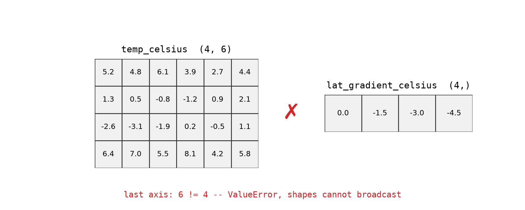
Figure 6:Broadcasting aligns shapes from the last axis backwards: 6 against 4 does not match, so temp_celsius + lat_gradient_celsius raises a ValueError.
# broadcasting: a (4,1) column stretches across the 6 longitudes
lat_gradient_celsius = np.array([0.0, -1.5, -3.0, -4.5])   # colder toward the north
adjusted = temp_celsius + lat_gradient_celsius[:, None]    # (4,1) + (4,6) -> (4,6)
print(adjusted.shape)
print(adjusted)
(4, 6)
[[ 5.2 4.8 6.1 3.9 2.7 4.4]
[-0.2 -1. -2.3 -2.7 -0.6 0.6]
[-5.6 -6.1 -4.9 -2.8 -3.5 -1.9]
[ 1.9 2.5 1. 3.6 -0.3 1.3]]
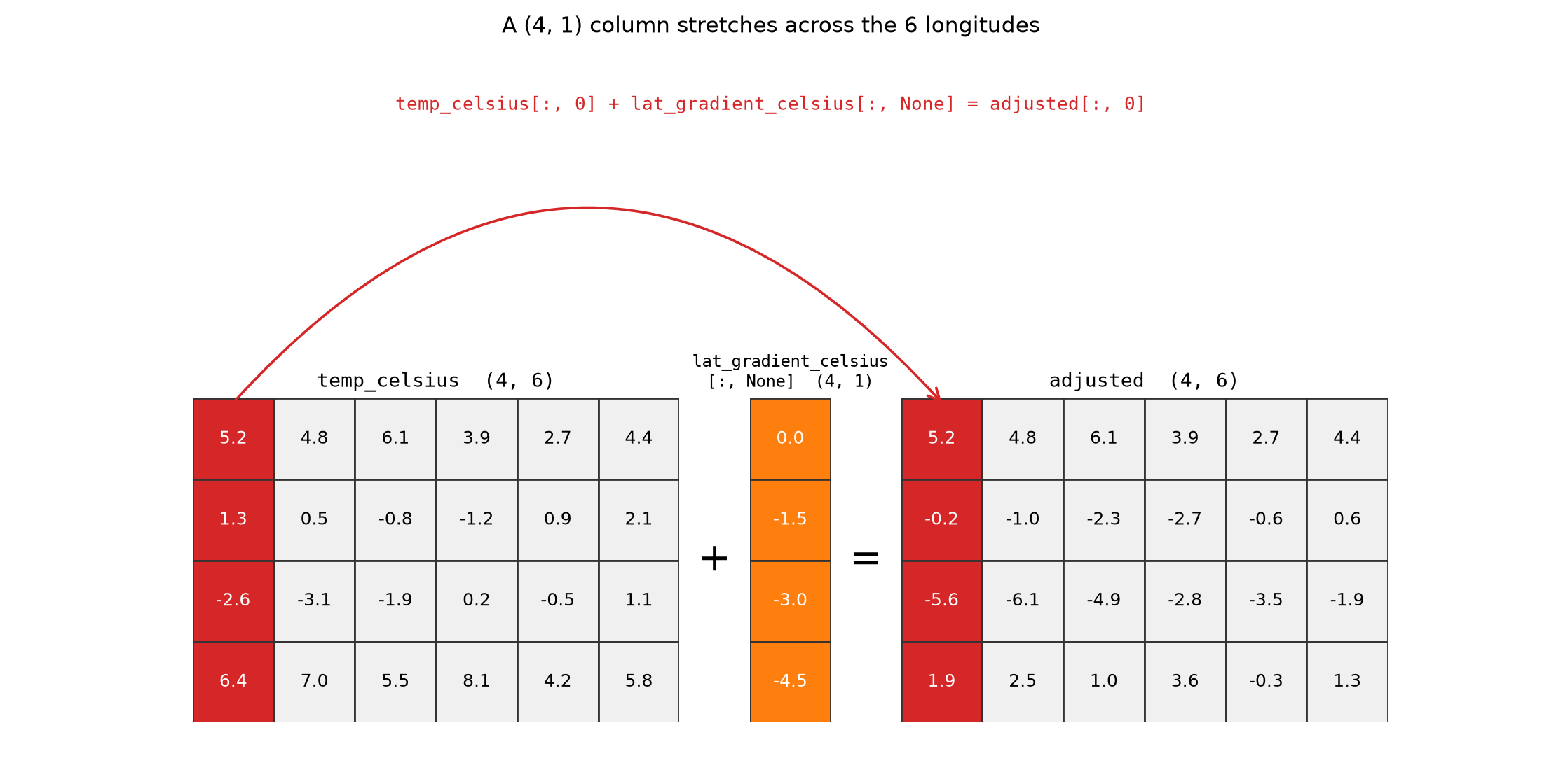
Figure 7:The (4, 1) column stretches across all 6 longitudes to combine with the (4, 6) field. (In linear-algebra notation this is A + b·1ᵀ: the column b repeated across every column via an outer product with a row of ones.)
Going deeper: vectorisation vs loops
Vectorised array operations run in compiled code and are typically one to two orders of magnitude faster than an equivalent Python loop. You can measure it in a notebook:
big = np.random.random(1_000_000)
%timeit big + 1.0                       # vectorised
%timeit [x + 1.0 for x in big]          # Python loop, much slower
The gap widens with array size. Reach for the array expression first; drop to a loop only when no vectorised form exists.
1.3.5 Calling functions on arrays
Most numpy operations are available two ways: as a method on the array (arr.mean()) or as a function in the numpy namespace (np.mean(arr)). They do the same thing — pick whichever reads more clearly.
print(temp_celsius.mean(), np.mean(temp_celsius))   # method and function agree
print(temp_celsius.sum(), np.sum(temp_celsius))
2.504166666666667 2.504166666666667
60.1 60.1
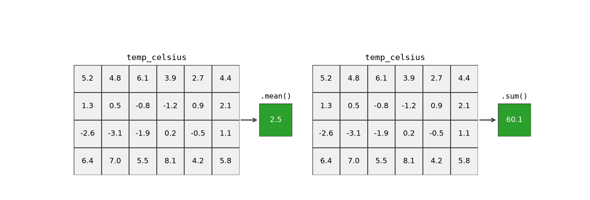
Figure 8:.mean() and .sum() with no axis collapse the whole array to one scalar.
Going deeper: other useful numpy functions
numpy provides element-wise maths and helpers for tidying values. A few you will reach for often:
a = np.array([1.234, -2.5, 9.876])
print(a.round(2))          # round to 2 decimals: [ 1.23 -2.5   9.88]
print(np.abs(a))           # absolute value
print(np.sqrt([1, 4, 9]))  # element-wise square root: [1. 2. 3.]
print(np.clip(a, 0, 5))    # limit values to the range [0, 5]
print(np.allclose([1.0, 2.0], [1.0, 2.0000001]))   # True — element-wise float comparison
round is useful for readable output, but it is only for display — keep full precision inside a calculation. np.allclose is the array version of the math.isclose you met in 1.1: never compare float
arrays with ==.
1.3.6 Reductions, reshape, and stacking
A reduction collapses an axis: axis=0 aggregates over latitudes (one result per longitude), axis=1 over longitudes. reshape reorganises the same data; stacking combines arrays.
Common reductions all take an optional axis:
| Function | Returns |
|---|---|
sum, mean, std | total, average, spread |
min, max | smallest / largest value |
argmin, argmax | index of the smallest / largest value |
cumsum, cumprod | running total / product |
# a reduction collapses an axis: axis=0 over rows, axis=1 over columns
print("overall mean:", temp_celsius.mean())
print("mean per column (over rows):", temp_celsius.mean(axis=0))
print("mean per row (over columns):", temp_celsius.mean(axis=1))
print("min, max:", temp_celsius.min(), temp_celsius.max())
print("argmin, argmax (flat index):", temp_celsius.argmin(), temp_celsius.argmax())

# reshape: same 24 values, new shape; -1 infers the missing length
flat = temp_celsius.reshape(-1)
print("reshaped:", flat.shape)

# stacking: combine arrays along a new row axis
col_means = temp_celsius.mean(axis=0)
index_row = np.arange(6, dtype=float)
print("vstacked:", np.vstack([index_row, col_means]).shape)
overall mean: 2.504166666666667
mean per column (over rows): [2.575 2.3 2.225 2.75 1.825 3.35 ]
mean per row (over columns): [ 4.51666667 0.46666667 -1.13333333 6.16666667]
min, max: -3.1 8.1
argmin, argmax (flat index): 13 21
reshaped: (24,)
vstacked: (2, 6)
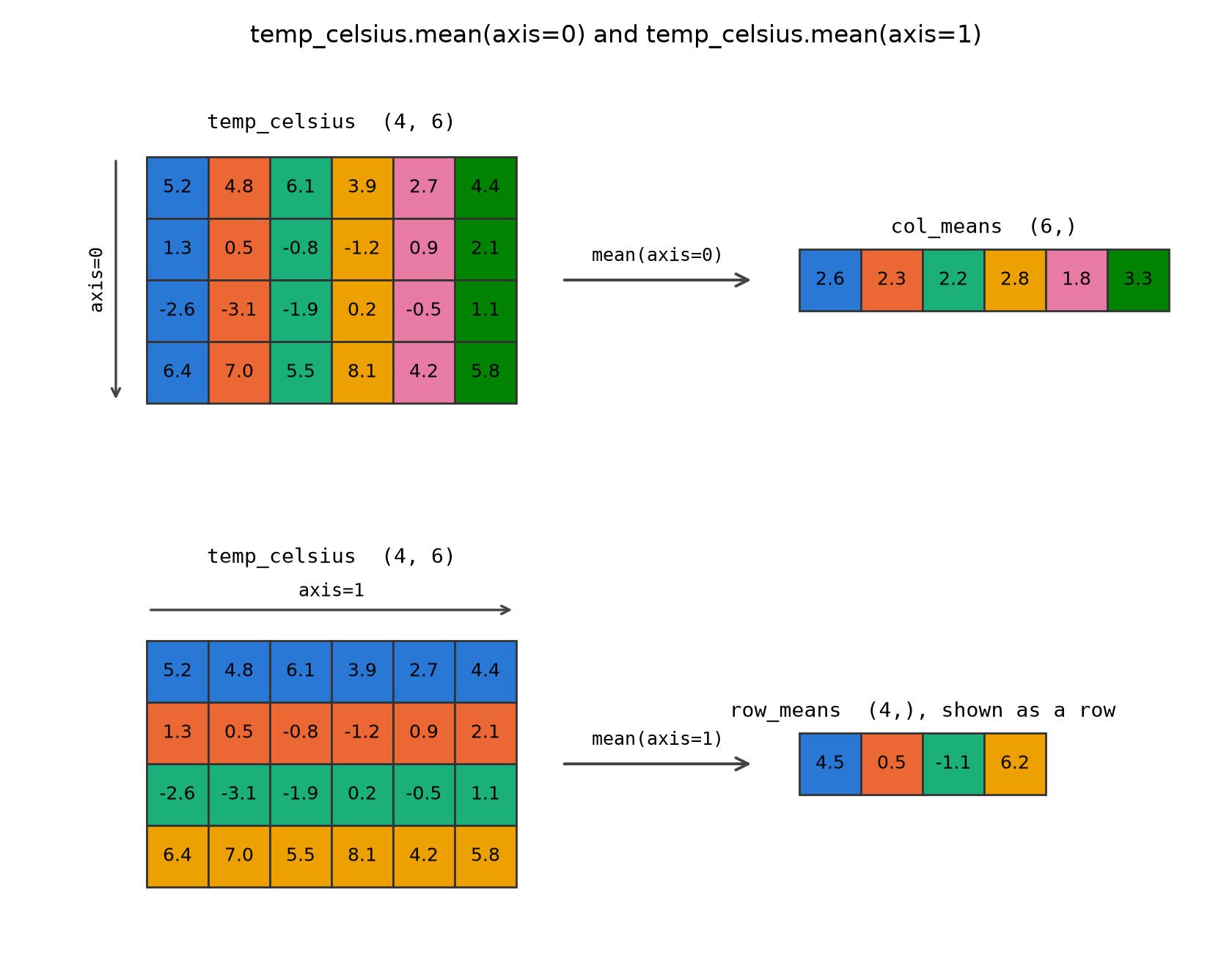
Figure 9:mean(axis=0) collapses the 4 rows to one value per column; mean(axis=1) collapses the 6 columns to one value per row (shown here as a row too, for comparison).
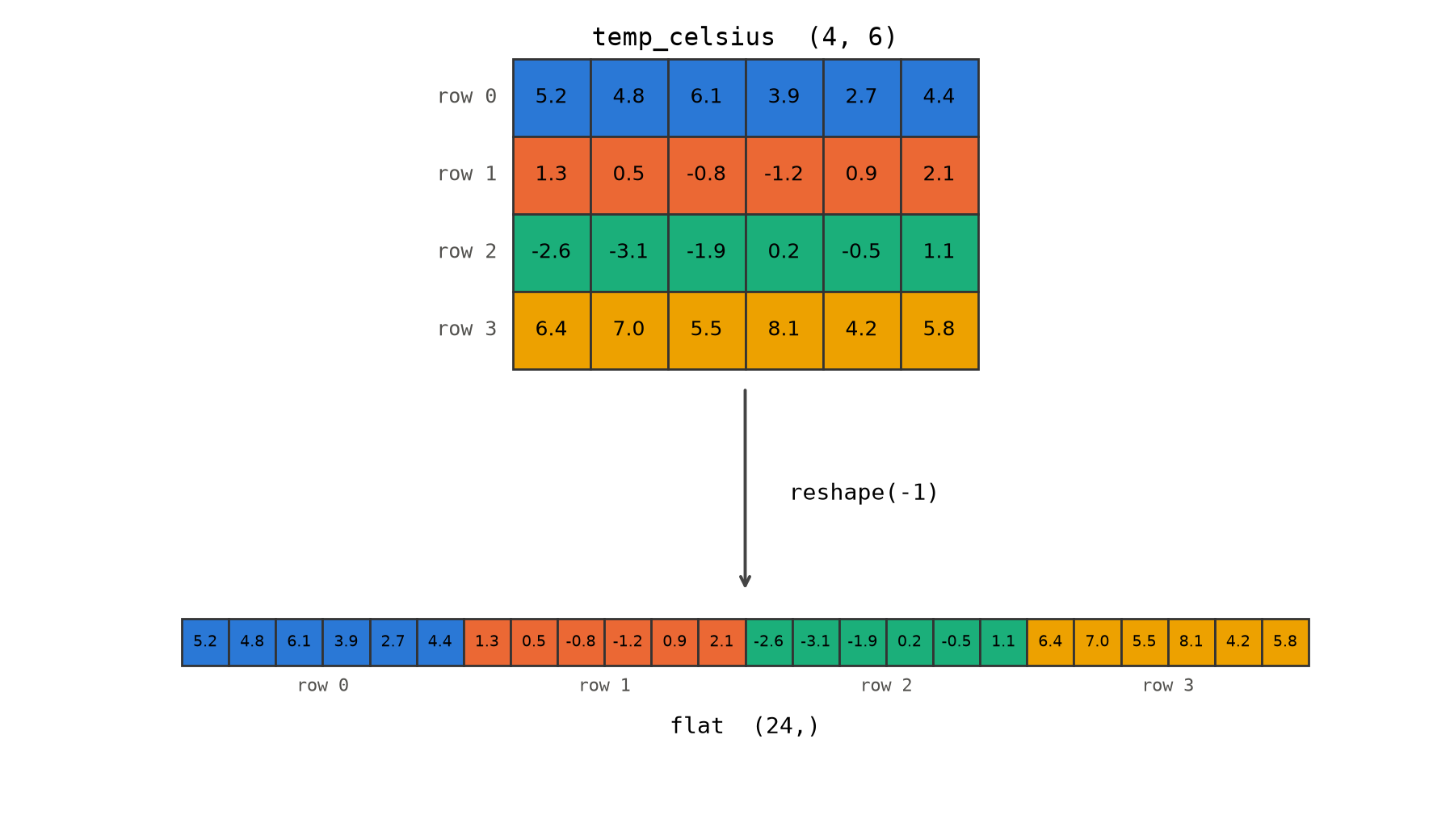
Figure 10:reshape(-1) reorganises the same 24 values into one flat row; nothing is recomputed.
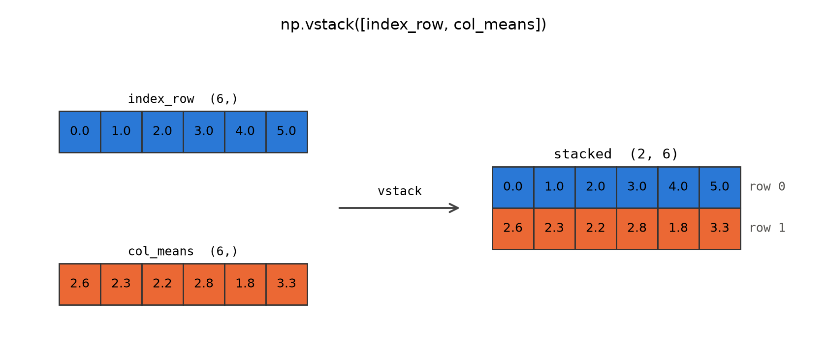
Figure 11:np.vstack([index_row, col_means]) stacks two (6,) rows into one (2, 6) array.
cumsum and cumprod are the exceptions in the table: they keep every partial result instead of collapsing the axis, so the output has the same shape as the input. For daily rainfall, the cumulative sum is the rain to date:
daily_rain_mm = np.array([0.0, 2.5, 0.0, 7.0, 1.5])
print(daily_rain_mm.cumsum())                  # [ 0.   2.5  2.5  9.5 11. ] — rain to date
print(daily_rain_mm.sum())                     # 11.0 — only the final total

# on a 2D field, axis works as for any reduction
print(temp_celsius.cumsum(axis=1).shape)       # (4, 6): a running total along each row
[ 0. 2.5 2.5 9.5 11. ]
11.0
(4, 6)
Solution
row_means = temp_celsius.mean(axis=1)
print(row_means)
print(int(row_means.argmax()))
Going deeper: basic linear algebra
numpy covers the everyday linear algebra a model needs.
A = np.array([[2.0, 1.0], [1.0, 3.0]])
b = np.array([1.0, 2.0])
print(A @ b)                 # matrix-vector product (also np.matmul)
print(np.linalg.solve(A, b)) # solve A x = b without inverting A
Prefer np.linalg.solve over forming np.linalg.inv(A) @ b: it is more accurate and faster.
1.3.7 Choosing, missing data, and interpolation
np.where picks element-wise between two options. Missing data is represented by NaN; np.isnan flags which elements are missing, NaN-aware reductions (np.nanmean, …) skip them, and ordinary reductions propagate NaN instead. np.interp fills a 1D gap by linear interpolation.
# np.where(condition, a, b): element-wise choice
category = np.where(temp_celsius < 0.0, "freezing", "above")
print(category)

# missing data as NaN; nan-aware vs ordinary reduction
temp_with_gaps = temp_celsius.copy()
temp_with_gaps[0, 0] = np.nan
print("nanmean (skips gaps):", np.nanmean(temp_with_gaps))
print("plain mean is contaminated:", np.mean(temp_with_gaps))  # nan
print("n missing:", np.isnan(temp_with_gaps).sum())      # np.isnan flags them; True counts as 1

# np.interp: fill a 1D gap by linear interpolation against an index
profile = temp_celsius[:, 0].copy()      # the first column, 4 latitudes
x = np.arange(profile.size)
known = np.array([0, 1, 3])              # pretend index 2 is missing
filled = np.interp(x, known, profile[known])
print(profile)
print(filled)                            # index 2 interpolated from its neighbours
[['above' 'above' 'above' 'above' 'above' 'above']
['above' 'above' 'freezing' 'freezing' 'above' 'above']
['freezing' 'freezing' 'freezing' 'above' 'freezing' 'above']
['above' 'above' 'above' 'above' 'above' 'above']]
nanmean (skips gaps): 2.38695652173913
plain mean is contaminated: nan
n missing: 1
[ 5.2 1.3 -2.6 6.4]
[5.2 1.3 3.85 6.4 ]
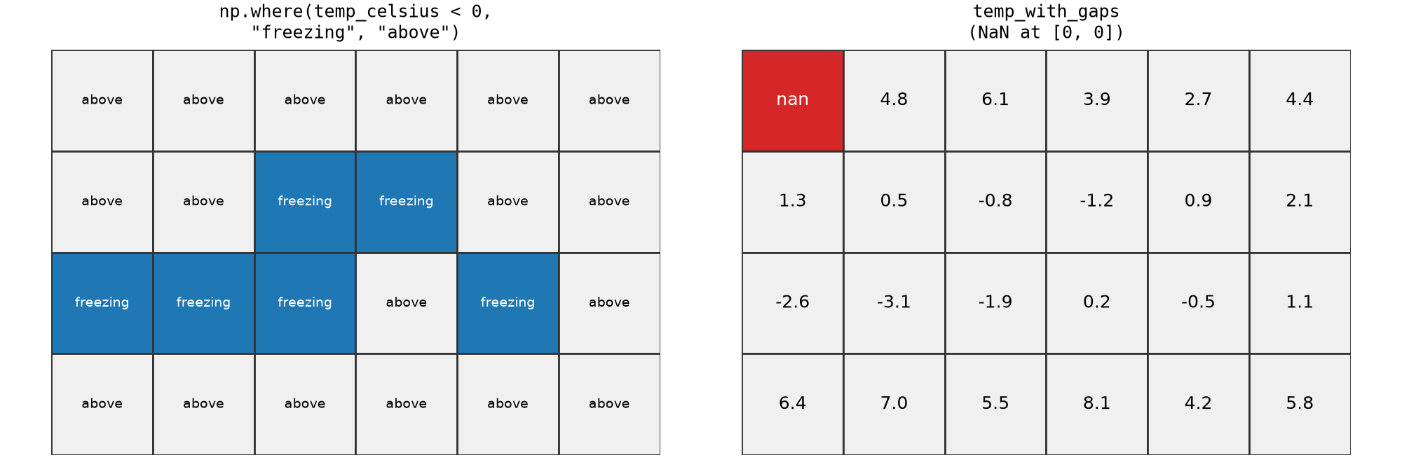
Figure 12:np.where(temp_celsius < 0, "freezing", "above") labels every cell; a NaN marks a missing one, propagating through an ordinary .mean() but skipped by np.nanmean().
~ flips a boolean mask, turning every True into False and back. Applied to np.isnan, it flags the values that are present, and indexing with that mask keeps only the real measurements, which are the values np.nanmean averages:
present = ~np.isnan(temp_with_gaps)            # True where a value exists
print("n present:", present.sum(), "of", temp_with_gaps.size)
print(np.allclose(temp_with_gaps[present].mean(), np.nanmean(temp_with_gaps)))   # True
n present: 23 of 24
True
1.3.8 Saving and loading arrays
numpy can write an array to disk in its own binary format, .npy, and read it back exactly as
it was — shape, dtype, and all. This is handy for intermediate results.
from pathlib import Path
Path("_files").mkdir(exist_ok=True)      # _files/ is not committed, so create it first

np.save("_files/temp_field.npy", temp_celsius)          # writes temp_field.npy

reloaded = np.load("_files/temp_field.npy")
print(reloaded.shape, reloaded.dtype)
print(np.allclose(temp_celsius, reloaded))       # True — an exact round trip
(4, 6) float64
True
Going deeper: bigger-than-memory arrays with dask
When a field is too large for memory, dask.array exposes the same numpy interface over chunks, building a task graph that runs only when you call .compute().
import dask.array as da
x = da.from_array(np.arange(1_000_000), chunks=100_000)
result = (x + 1).mean()      # lazy: nothing computed yet
print(result.compute())      # runs the graph, chunk by chunk
xarray uses this same lazy, chunked model for climate-scale datasets in later subchapters.
When generated code lies: a silent dtype truncation
AI assistants often preallocate an output array with np.zeros_like, which copies the input’s dtype. If the input is integer, float results are silently truncated on assignment. Here a function computes anomalies (value minus the field mean) for an integer precipitation field.
def to_anomaly(field):
    # subtract the mean into a preallocated array (as an assistant returned it)
    result = np.zeros_like(field)        # inherits field's dtype!
    result[:] = field - field.mean()
    return result

precip_mm = np.array([[0, 2, 5], [1, 0, 8], [3, 4, 2]])   # integer mm
print("input dtype:", precip_mm.dtype)
print(to_anomaly(precip_mm))
input dtype: int64
[[-2 0 2]
[-1 -2 5]
[ 0 1 0]]
def to_anomaly(field):
    # let numpy promote to float; no wrong-dtype preallocation
    return field - field.mean()

print(to_anomaly(precip_mm))
print("output dtype:", to_anomaly(precip_mm).dtype)
[[-2.77777778 -0.77777778 2.22222222]
[-1.77777778 -2.77777778 5.22222222]
[ 0.22222222 1.22222222 -0.77777778]]
output dtype: float64
Summary
| Concept | Rule to remember |
|---|---|
| Arrays | One dtype and one shape; build them with np.array, zeros, ones, arange, linspace. |
| Indexing | [row, col] selects, boolean masks filter; a slice is a view, .copy() makes it independent. |
| Vectorising | Write array expressions instead of element-by-element loops. |
| Broadcasting | Shapes align from the last axis backwards; [:, None] adds a length-1 axis. |
| Reductions | State the axis explicitly (mean, sum, min, max, argmin, argmax). |
| Missing data | np.where chooses element-wise, np.isnan detects, np.interp fills 1D gaps. |
| dtype | np.zeros_like(int_array) truncates float results silently — let numpy promote to float. |
Resources
NumPy: the absolute basics for beginners — numpy’s own official introduction, covering the same array-creation, indexing, and broadcasting ideas as this notebook.
Python Data Science Handbook — Introduction to NumPy — free online; thorough coverage of arrays, broadcasting, masking, and ufuncs.
Scientific Python Lectures — NumPy — a concise, research-oriented tour of array creation, operations, and reductions.