Exercises - MLEES

Exercise 1: Create and inspect¶

Build the following 3×4 field of temperatures (°C) as a numpy array:

5.2 4.8 6.1 3.9 1.3 0.5 -0.8 -1.2 -2.6 -3.1 -1.9 0.2

Print its shape, ndim, and dtype, and its overall mean rounded to two decimals. Then create, and print, three arrays of the same shape without typing the shape out by hand: all ones, a uniform reference field of 15.0 °C, and random values in [0, 1).

# Your solution here

Exercise 2: Index and slice¶

Given

a = np.array([[1.0, 2.0, 3.0, 4.0],
              [5.0, 6.0, 7.0, 8.0],
              [9.0, 10.0, 11.0, 12.0]])

print the last row, the first column, and the 2×2 sub-block formed by the first two rows and the last two columns.

Finally, take a slice of the first row, change its first element to 99.0, and print the original array. Then repeat using .copy(). Explain the difference in a comment.

# Your solution here

Exercise 3: Masking and np.where¶

Given

temp_celsius = np.array([[-1.0, 12.0,  3.0],
                         [ 8.0, -2.0, 15.0],
                         [ 4.0,  0.5, 11.0]])

print the values that exceed 10 °C, their mean, and the percentage of the field they make up. Then build a clipped field in which every value below 0 °C is set to 0, using np.where.

# Your solution here

Exercise 4: Broadcasting and grids¶

Given the field below, add a per-column offset (length 4) to every row, and separately add a per-row offset (length 3) to every column.

field = np.array([[1.0, 2.0, 3.0, 4.0],
                  [5.0, 6.0, 7.0, 8.0],
                  [9.0, 10.0, 11.0, 12.0]])
col_offset = np.array([0.0, 1.0, 2.0, 3.0])
row_offset = np.array([10.0, 20.0, 30.0])

Then build a grid of 4 evenly spaced longitudes from 6 to 9 °E and 3 evenly spaced latitudes from 46 to 47 °N, so that it has the same shape as field. On that grid, compute a synthetic temperature field that is 15.0 °C at (6 °E, 46 °N), cools by 0.6 °C per degree of latitude northward, and warms by 0.2 °C per degree of longitude eastward. Compute it twice, once from the 2D arrays that np.meshgrid returns and once by broadcasting the 1D latitudes and longitudes directly, and confirm with np.allclose that the two agree.

# Your solution here

Exercise 5: Axis reductions¶

Given seasonal mean temperatures at three stations, one row per station and one column per season (winter, spring, summer, autumn):

seasonal_celsius = np.array([[ 2.1,  9.8, 18.4, 10.2],
                             [-1.5,  7.2, 16.9,  8.0],
                             [ 4.0, 11.5, 20.3, 12.6]])

print the annual mean at each station and the index of each station’s warmest season. Then find the coldest value in each season twice, once with the method and once with the numpy function, and confirm they agree.

Finally, given four days of rainfall at two stations, one row per station,

rain_mm = np.array([[0.0, 6.2, 1.1, 0.0],
                    [2.4, 0.0, 0.0, 8.3]])

use cumsum along the right axis to get the rain to date. Print the index of the station that was wetter after the second day and the index of the station that was wetter after all four. Are they the same station?

# Your solution here

Exercise 6: Missing data and interpolation¶

Given hourly air temperatures with a gap of two readings,

temp_celsius = np.array([12.0, 13.5, np.nan, np.nan, 18.0, 18.5])

fill the gap by linear interpolation against the integer index. Then print the NaN-aware mean of the original series and the ordinary mean of the filled one. The two differ; say in a comment why.

# Your solution here

Exercise 7: Avoid the dtype trap¶

An assistant wrote this function to compute each cell’s share of the total rainfall in an integer field of rain-gauge readings:

def rain_share(rain_mm):
    share = np.zeros_like(rain_mm)
    share[:] = rain_mm / rain_mm.sum()
    return share

rain_mm = np.array([[0, 2, 5], [1, 0, 8], [3, 4, 2]])

Call it and print the result. Explain in a comment why every share is 0, then fix the function twice: once keeping the preallocation but passing dtype=float to np.zeros_like, and once without preallocating at all. Confirm that each fixed version returns a float array whose shares sum to 1.

# Your solution here

Exercise 8: Reshape and stack¶

Create the integers 0 to 11 as a 1D array, then reshape it into a 3×4 array and print both shapes.
Reshape the same data into a 4×3 array. Print it and say in a comment why the numbers appear in a different arrangement.
Use reshape(-1) to flatten your 3×4 array back to 1D, and confirm the shape.
Stack the 3×4 array on top of a row of zeros with np.vstack, and print the resulting shape.

# Your solution here

Exercise 9: Ocean float profiles¶

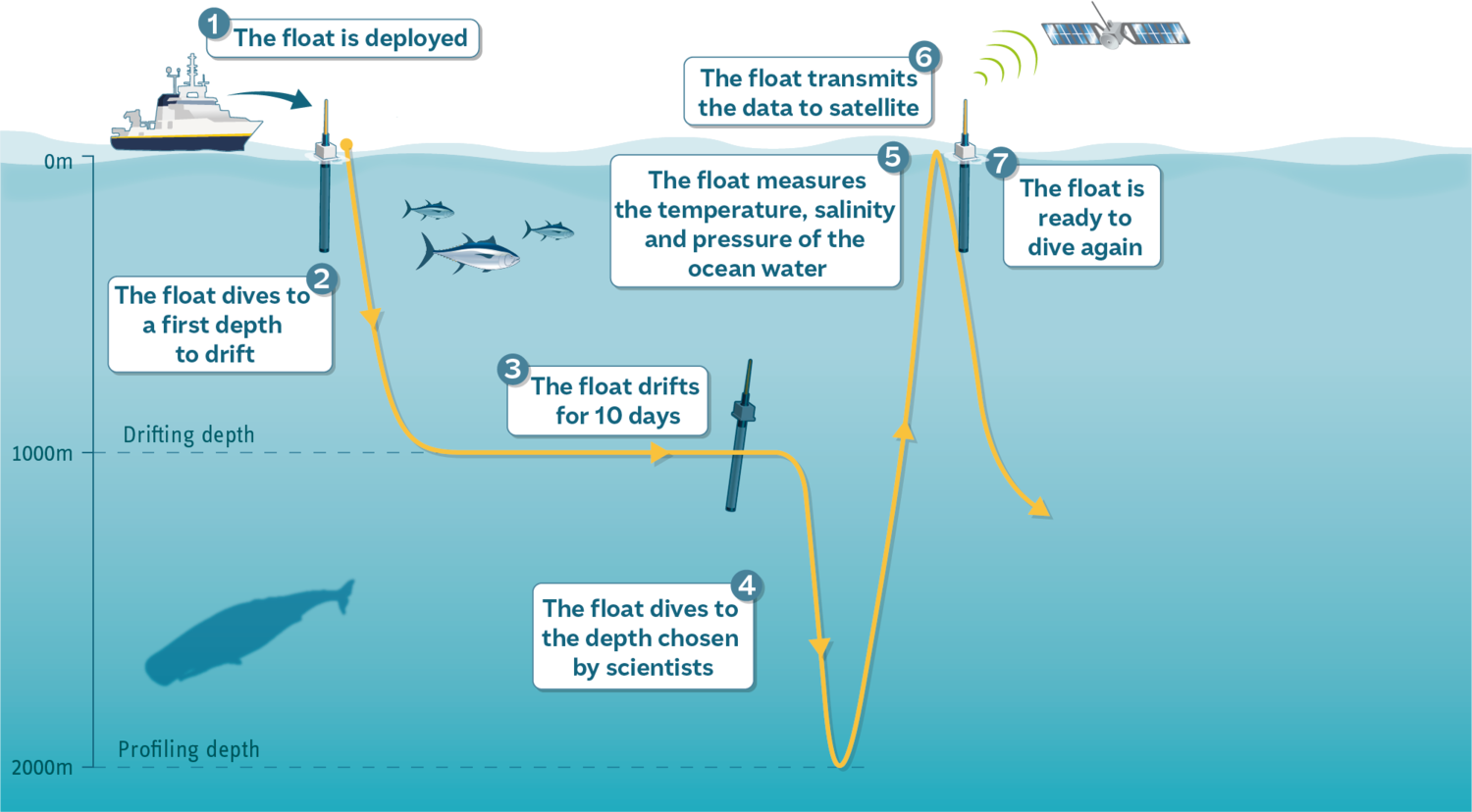
A diagram of one Argo float cycle, numbered one to seven, from deployment through drift, dive, ascent and satellite transmission — Figure 1:One cycle of an Argo float: deployment, descent to a drifting depth of about 1000 m, ten days of drift, a dive to the profiling depth, then the ascent during which the measurements are taken, and transmission to satellite at the surface before the next cycle begins. The panel on the right shows what one ascent produces — the temperature and salinity profiles you are about to work with. Illustration © Thomas Haessig, from Euro-Argo ERIC’s educational material.

Argo floats are autonomous instruments that drift with ocean currents, periodically diving and surfacing while recording temperature, salinity, and pressure. Each dive produces one profile: a set of measurements at many depth levels, with a single latitude, longitude, and date attached.

This exercise uses real Argo data. Steps 1 to 8 use only what 1.1 to 1.3 cover: loading arrays, inspecting shapes, rebuilding an axis, vectorised arithmetic, reductions along an axis, boolean masks, and NaN-aware statistics. Steps 9 to 11 then plot what you computed.

# Pre-supplied: download and unzip the Argo data files.
import pooch

files = pooch.retrieve(
    url="https://raw.githubusercontent.com/gse-unil/2026_MLEES_book/main/data/part-I/argo_float_data.zip",
    known_hash="sha256:dd913ba3450241bcd5d5697187ea68d398bdd7fd563a04cc74386834749c25f5",
    processor=pooch.Unzip(),
    path=pooch.os_cache("mlees"),
)
for f in sorted(files):
    print(f)

/home/runner/.cache/mlees/3447957d2e428811e6534de5c131c0db-argo_float_data.zip.unzip/P.npy
/home/runner/.cache/mlees/3447957d2e428811e6534de5c131c0db-argo_float_data.zip.unzip/S.npy
/home/runner/.cache/mlees/3447957d2e428811e6534de5c131c0db-argo_float_data.zip.unzip/T.npy
/home/runner/.cache/mlees/3447957d2e428811e6534de5c131c0db-argo_float_data.zip.unzip/date.npy
/home/runner/.cache/mlees/3447957d2e428811e6534de5c131c0db-argo_float_data.zip.unzip/lat.npy
/home/runner/.cache/mlees/3447957d2e428811e6534de5c131c0db-argo_float_data.zip.unzip/levels.npy
/home/runner/.cache/mlees/3447957d2e428811e6534de5c131c0db-argo_float_data.zip.unzip/lon.npy

Step 1. Load each .npy file into a numpy array with np.load. Name them T (temperature, °C), S (practical salinity, unitless), P (pressure, dbar), date, lat, lon, and level (depth level).

Read the filenames printed above to work out which file is which.

# Your solution here
# Hint: every file sits in the same folder, Path(files[0]).parent (Path comes from pathlib)
# Hint: join a filename onto that folder with /, as in Path("_files") / "station_daily.csv"
# Hint: np.load(path) returns the array stored in a .npy file

Step 2. Print the shape of every array you loaded. Then answer in a comment: which dimension do T, S, and P share with level, and which do they share with lat, lon, and date?

# Your solution here
# Hint: the profile arrays are two-dimensional; the coordinate arrays are one-dimensional
# Hint: a 2D array's shape tells you the length of each axis — match those against the 1D shapes

Step 3. The level array is a regular sequence. Recreate it twice — once with np.arange and once with np.linspace — and confirm each matches the original using np.allclose.

Read level[0], level[-1], and level.size first to work out the arguments.

# Your solution here
# Hint: np.arange(start, stop, step) excludes the stop value
# Hint: np.linspace(start, stop, num) includes both ends
# Hint: np.allclose(a, b) returns True when every pair of elements is close enough

Step 4. Compute the density of seawater relative to pure water, in kg m⁻³:

\rho - \rho_{\text{pure water}} = a\,S + b\,\Theta + c\,\Theta^{2}

(1)

where $S$ is salinity and $\Theta$ is the conservative temperature, computed from temperature, salinity, and pressure by the gsw library. The constants are

a = 7.718e-1
b = -8.44e-2
c = -4.561e-3

The cell below imports the function. Compute conservative_temp and relative_density, print the shape of your result, and check it matches T.

Both CT_from_t and the formula expect absolute salinity, in g/kg, while Argo reports practical salinity, which has no unit. Absolute salinity is about 0.5 % larger; for these profiles, using practical salinity in its place lowers every relative density by about 0.13 kg m⁻³, which is small enough to ignore here. gsw.SA_from_SP does the exact conversion when it matters.

Source: Roquet et al. (2015), J. Phys. Oceanogr. 45, 2564–2579, and the TEOS-10 GSW toolbox.

# Pre-supplied: the conservative-temperature function from the gsw library
from gsw import CT_from_t

# Your solution here
# Hint: CT_from_t(SA, t, p) takes salinity, temperature, and pressure — in that order
# Hint: the whole formula is one vectorised expression; no loop is needed
# Hint: Theta**2 squares every element

Step 5. Compute the mean and the standard deviation of T, S, P, and relative_density at each depth, averaging across all the profiles.

Check your result has the same shape as level — if it does not, you reduced along the wrong axis.

# Your solution here
# Hint: pick the axis that runs across profiles, not across depths
# Hint: mean_T.shape should equal level.shape

Step 6. Look at the mean you just computed. Many entries are nan, because Argo profiles contain missing values and an ordinary mean propagates them.

Count how many values in T are missing, using np.isnan and a sum over the boolean mask.
Express that as a percentage of all values in T.
Recompute the mean and standard deviation with np.nanmean and np.nanstd, and confirm no nan remains.

# Your solution here
# Hint: np.isnan(T) gives a boolean array; True counts as 1 when summed
# Hint: T.size is the total number of elements
# Hint: np.isnan(result).sum() counts the nan that survived; it should be 0

Step 7. Using np.where, build an array that labels each depth "warm" where the mean temperature there is above 10 °C and "cold" otherwise. Print the first ten labels alongside the first ten depths.

Then, using a boolean mask, print the depths at which the mean temperature is below 5 °C.

# Your solution here
# Hint: np.where(condition, value_if_true, value_if_false) works element-wise
# Hint: level[mask] selects the depths where the mask is True

Step 8. Assemble a summary array with np.vstack: one row of depths, one of mean temperature, one of mean salinity, and one of mean relative density — four rows in total.

Print its shape, save it to _files/argo_summary.npy, load it back, and confirm with np.allclose that the round trip changed nothing.

# Your solution here
# Hint: np.vstack takes a list of 1D arrays and stacks them as rows
# Hint: your summary should have shape (4, n_levels)
# Hint: _files/ may not exist yet; create it first with Path("_files").mkdir(exist_ok=True)

Step 9. Plot each of T, S, P and relative_density against depth — four figures, one per variable.

Each array is (level, profile), so handing the whole array to plt.plot draws one line per profile. Put the variable on the x-axis and level on the y-axis, which is the oceanographic convention: depth runs down the page, and a profile is read the way the float measured it.

It will look messy, because 75 profiles are drawn on top of each other.

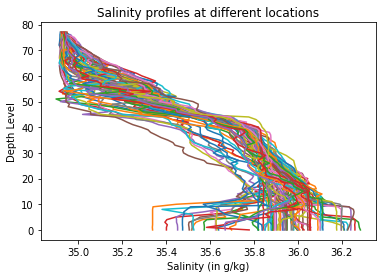
Many overlapping salinity profiles plotted against depth level, forming a dense band that shifts towards fresher water with depth — Figure 2:The salinity panel, as a check on yours. Label the axes and give each figure a title.

# Your solution here
# Hint: plt.figure() before each variable's plot, plt.show() after it
# Hint: plt.plot(S, level) draws one line per column of S
# Hint: the semicolon at the end of a plt.plot call suppresses the list of line objects
# Hint: plt.xlabel, plt.ylabel and plt.title each take a string

Step 10. Now plot only the mean profile of each variable, with the standard deviation as error bars.

Use the NaN-aware mean and standard deviation from Step 6, and draw them with plt.errorbar. Because the variable is on the x-axis, the spread is a horizontal error bar — the keyword is xerr, not yerr.

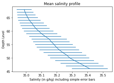
Figure 3:The salinity panel again, reduced from 75 profiles to one line and its spread.

In a comment, say what the width of the error bars tells you about how much the profiles disagree near the surface compared with at depth.

# Your solution here
# Hint: plt.errorbar(mean_S, level, xerr=std_S)
# Hint: use the nan-aware versions from Step 6, or every bar will be missing

Step 11. Scatter the profiles’ longitudes against their latitudes.

One point per profile. Label both axes and give it a title, and set the marker size with s= so the points are readable. Then print the first three entries of date and the last one.

In a comment, say what the dates and the shape of the cloud tell you about how this set of profiles was collected, and by how many floats.

# Your solution here
# Hint: plt.scatter(lon, lat)
# Hint: lon and lat have one entry per profile, not per level
# Hint: look at the spacing between consecutive dates