

geopandas extends the pandas dataframe with a geometry column and a coordinate reference system (crs), so points, lines, and polygons can be filtered, joined, measured, and mapped with familiar syntax. This subchapter builds a small set of Swiss weather stations and hazard zones, reprojects between the geographic crs WGS84 (EPSG:4326) and the projected Swiss crs LV95 (EPSG:2056), and works through spatial joins, buffers, dissolves, and overlays. At the end, the generated code measures distance and area in degrees instead of a projected crs — the single most common geospatial mistake.

Figure 1:The geopandas logo, from the project’s own documentation.
1.6.1 GeoDataFrame and shapely Geometries
A GeoDataFrame is a pandas DataFrame with an active geometry column of shapely objects (Point, LineString, Polygon) and an attached crs. The crs states how the coordinates map to the Earth; without it, they are numbers in an arbitrary plane.
import geopandas as gpd
from shapely.geometry import Point, Polygon, LineString

stations = gpd.GeoDataFrame(
    {"name": ["Basel", "Zurich", "Bern", "Lugano"]},
    geometry=[Point(7.59, 47.56), Point(8.54, 47.37),
              Point(7.44, 46.95), Point(8.95, 46.00)],
    crs="EPSG:4326",   # WGS84 longitude/latitude in degrees
)
print(stations)
print("crs:", stations.crs.to_epsg(), "| geometry type:", stations.geom_type.iloc[0])
name geometry
0 Basel POINT (7.59 47.56)
1 Zurich POINT (8.54 47.37)
2 Bern POINT (7.44 46.95)
3 Lugano POINT (8.95 46)
crs: 4326 | geometry type: Point
1.6.2 Reading and Writing Vector Formats
geopandas reads and writes shapefiles (.shp), GeoJSON (.geojson), and GeoPackage (.gpkg) through read_file/to_file. GeoPackage is a single-file, modern default; a shapefile is really several files and has column-name and size limits.
from pathlib import Path

Path("_files").mkdir(exist_ok=True)
stations.to_file("_files/stations.geojson", driver="GeoJSON")
stations.to_file("_files/stations.gpkg", driver="GPKG")

reread = gpd.read_file("_files/stations.gpkg")
print("reread shape:", reread.shape, "| crs preserved:", reread.crs.to_epsg())
reread shape: (4, 2) | crs preserved: 4326
# a shapefile round-trip, written and read the same way as GeoJSON/GeoPackage above
stations.to_file("_files/stations.shp")   # driver inferred from the .shp extension
reread_shp = gpd.read_file("_files/stations.shp")
print("reread shape:", reread_shp.shape, "| crs preserved:", reread_shp.crs.to_epsg())

# a shapefile is not one file: this write also creates _files/stations.shx, .dbf, .prj (and more)
print("shapefile sidecar files:", sorted(p.name for p in Path("_files").glob("stations.*")))
reread shape: (4, 2) | crs preserved: 4326
shapefile sidecar files: ['stations.cpg', 'stations.dbf', 'stations.geojson', 'stations.gpkg', 'stations.prj', 'stations.shp', 'stations.shx']
1.6.3 Coordinate Reference Systems and Reprojection
Inspect the crs with .crs; change it with to_crs. Reprojecting from geographic WGS84 to the projected Swiss system LV95 (EPSG:2056) converts degrees to metres, which is what makes metric measurement meaningful.
stations_lv95 = stations.to_crs(2056)   # reproject to metric Swiss coordinates

print("before:", stations.crs.to_epsg(), "->", "after:", stations_lv95.crs.to_epsg())
print("Basel WGS84 (deg):", round(stations.geometry.x.iloc[0], 3), round(stations.geometry.y.iloc[0], 3))
print("Basel LV95 (m):  ", round(stations_lv95.geometry.x.iloc[0], 1), round(stations_lv95.geometry.y.iloc[0], 1))
before: 4326 -> after: 2056
Basel WGS84 (deg): 7.59 47.56
Basel LV95 (m): 2611393.1 1267709.5
1.6.4 Spatial Predicates and Joins
Spatial predicates (within, intersects, contains) test topological relationships. A spatial join (sjoin) attaches attributes from one layer to another by location rather than by a shared key.
zones = gpd.GeoDataFrame(
    {"hazard": ["flood", "flood"]},
    geometry=[Polygon([(7, 47), (8, 47), (8, 48), (7, 48)]),      # north-west box
              Polygon([(8, 47), (9, 47), (9, 48), (8, 48)])],     # north-east box
    crs="EPSG:4326",
)

# which stations fall within a hazard zone?
in_hazard = gpd.sjoin(stations, zones, predicate="within", how="inner")
print("stations in a hazard zone:", in_hazard["name"].tolist())
stations in a hazard zone: ['Basel', 'Zurich']
1.6.5 Buffer, Dissolve, Overlay, and Centroid
buffer grows a geometry by a distance (in crs units, so project first); dissolve merges geometries that share an attribute; overlay combines two layers by a set operation such as intersection; .centroid returns a single representative point for a polygon — handy for labelling a zone or measuring to it without carrying the whole shape around.
# buffer: a 20 km catchment around each station (metric crs required)
buffers = stations_lv95.buffer(20_000)
print("buffer area:", round(buffers.area.iloc[0] / 1e6, 1), "km^2")

# dissolve: merge the two flood boxes into one polygon by shared attribute
dissolved = zones.dissolve(by="hazard")
print("polygons after dissolve:", len(dissolved))

# centroid: a single representative point for the dissolved polygon
zone_centroid = dissolved.geometry.iloc[0].centroid
print("dissolved hazard-zone centroid:", round(zone_centroid.x, 3), round(zone_centroid.y, 3))

# overlay: intersection of the hazard zones with the Basel buffer
basel_buffer = gpd.GeoDataFrame(geometry=[buffers.iloc[0]], crs=2056)
clip = gpd.overlay(zones.to_crs(2056), basel_buffer, how="intersection")
print("overlay produced", len(clip), "piece(s), area",
      round(clip.area.sum() / 1e6, 1), "km^2")
buffer area: 1254.6 km^2
polygons after dissolve: 1
dissolved hazard-zone centroid: 8.0 47.5
overlay produced 1 piece(s), area 1254.6 km^2
# length: distance measured along a line, e.g. a straight-line route between two stations
route = LineString([stations_lv95.geometry.iloc[0], stations_lv95.geometry.iloc[2]])  # Basel -> Bern
print("Basel-Bern straight-line route length:", round(route.length / 1000, 1), "km")
Basel-Bern straight-line route length: 68.8 km
1.6.6 Plotting a Map
geopandas plots geometries directly on a matplotlib axes; layers are drawn by calling .plot() on the same axes. The cell below first flags each station with .isin(), which checks whether a value appears in a given list or Series — here, whether a station’s name is among the names already found inside a hazard zone.
%matplotlib inline
import matplotlib.pyplot as plt

flagged = stations.assign(in_hazard=stations["name"].isin(in_hazard["name"]))

fig, ax = plt.subplots(figsize=(5, 5))
zones.boundary.plot(ax=ax, color="tab:red", linewidth=1)
flagged.plot(ax=ax, column="in_hazard", categorical=True, legend=True, markersize=40)
ax.set_xlabel("longitude (°E)")
ax.set_ylabel("latitude (°N)")
ax.set_title("stations and hazard zones (EPSG:4326)")
plt.show()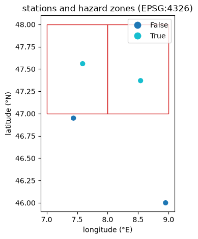
Solution
lv95 = stations.to_crs(2056)
basel = lv95.loc[lv95["name"] == "Basel", "geometry"].iloc[0]
bern = lv95.loc[lv95["name"] == "Bern", "geometry"].iloc[0]
print(round(basel.distance(bern) / 1000, 1), "km")
When generated code lies: measuring in degrees
Asked for the distance between two stations, an assistant calls .distance() on the data as loaded — in EPSG:4326. The result is a number of degrees, not metres. geopandas even warns, but the value looks plausible and flows on into whatever comes next.
# the "distance between two stations" as an assistant might compute it
import warnings

with warnings.catch_warnings(record=True) as caught:
    warnings.simplefilter("always")
    dist_deg = stations.geometry.distance(stations.geometry.iloc[2])   # Basel..Bern etc., in EPSG:4326
    area_deg = gpd.GeoSeries(
        [Polygon([(7, 47), (8, 47), (8, 48), (7, 48)])], crs="EPSG:4326").area

print("Basel->Bern distance in degrees (wrong):", round(dist_deg.iloc[0], 4))
print("1x1 degree box area in deg^2 (wrong):", round(area_deg.iloc[0], 4))
print("geopandas warned about a geographic crs:",
      any("geographic CRS" in str(warning.message) for warning in caught))

print(f'\n{caught[0].message}')
Basel->Bern distance in degrees (wrong): 0.6282
1x1 degree box area in deg^2 (wrong): 1.0
geopandas warned about a geographic crs: True
Geometry is in a geographic CRS. Results from 'distance' are likely incorrect. Use 'GeoSeries.to_crs()' to re-project geometries to a projected CRS before this operation.
dist_m = stations_lv95.geometry.distance(stations_lv95.geometry.iloc[2])
area_m2 = gpd.GeoSeries(
    [Polygon([(7, 47), (8, 47), (8, 48), (7, 48)])], crs="EPSG:4326").to_crs(2056).area

print("Basel->Bern distance:", round(dist_m.iloc[0] / 1000, 1), "km")
print("1x1 degree box area:", round(area_m2.iloc[0] / 1e6, 0), "km^2")
Basel->Bern distance: 68.8 km
1x1 degree box area: 8378.0 km^2
Going deeper: raster data with rioxarray
Vector data has geometries; raster data has a grid of cells (a digital elevation model, satellite imagery). rioxarray adds a crs and geotransform to an xarray DataArray.
import rioxarray
dem = rioxarray.open_rasterio("dem.tif")      # dims (band, y, x), with a crs
dem_lv95 = dem.rio.reproject("EPSG:2056")
The same crs discipline applies: reproject before measuring.
Going deeper: zonal statistics
Zonal statistics summarise raster values within vector polygons — for example the mean elevation of each catchment.
from rasterstats import zonal_stats
stats = zonal_stats("catchments.gpkg", "dem.tif", stats=["mean", "max"])
Zonal statistics is the usual way raster and vector data meet in a workflow: the vector polygon defines a zone, the raster supplies the values inside it.
Going deeper: slope and aspect from a DEM
Terrain derivatives come from the spatial gradient of an elevation grid. With a DEM as an array of elevations and a grid spacing dx, dy:
import numpy as np
dz_dy, dz_dx = np.gradient(elevation, dy, dx)
slope = np.arctan(np.hypot(dz_dx, dz_dy))     # radians
aspect = np.arctan2(-dz_dy, dz_dx)            # direction of steepest descent
Dedicated tools (richdem, gdaldem) handle edge effects and units more carefully.
Going deeper: interactive web maps with folium
GeoDataFrame.explore() builds a leaflet web map (via folium) for interactive inspection in a notebook.
stations.explore(column="name", tiles="OpenStreetMap")Useful for exploration; static matplotlib maps remain better for print figures.
Summary
| Concept | Rule to remember |
|---|---|
| GeoDataFrame | A DataFrame with a geometry column and a crs. |
| The crs | What gives coordinates physical meaning; read it with .crs, change it with to_crs. |
| Formats | read_file/to_file handle shp, geojson, and gpkg; prefer GeoPackage to shapefile. |
| Measuring | Area, length, and distance only in a projected metric crs — never in degrees. |
| Relating layers | Spatial predicates and sjoin join two layers by location. |
| Combining geometries | buffer (project first), dissolve (merge by attribute), overlay (set operations), .centroid. |
Resources
GeoPandas — Managing projections — setting and transforming coordinate reference systems, including why measurements require a projected crs.
GeoPandas basics: maps, projections, and spatial joins — a worked introduction to GeoDataFrames, crs handling, spatial joins, and plotting.