

This notebook builds a hierarchy of three models — a deterministic UNet, a variational autoencoder, and a latent diffusion model — that turns 25 km ERA5 2 m temperature fields into 2.2 km fields over Italy, following Tomasi et al. (2025) in a deliberately simplified form.
Run it on a GPU. Training the whole hierarchy takes roughly 45 minutes, so pretrained checkpoints ship with the data: the inference and scoring sections at the end can be run on their own.
# On Colab or Kaggle these packages are not installed by default; a local clone gets them
# from the project's own environment, so this cell does nothing there.
import sys

if "google.colab" in sys.modules or "kaggle_secrets" in sys.modules:
    # lightning is pinned below 2.6: the pretrained checkpoints store a live module and
    # omegaconf objects in their hyper-parameters, which 2.6 refuses to unpickle
    !pip install -q pooch "lightning>=2.5.3,<2.6" omegaconf properscoring zstandard rioxarray rasterio
The data
The data and the pretrained checkpoints come as one 1.94 GiB archive: a year (2020) of hourly
ERA5 and COSMO-CLM temperature fields over the Italian domain, the three static rasters, and the
three sets of checkpoints. pooch downloads it once, checks it against the sha256 below, and
unpacks it into a shared cache, so later runs reuse what is already on disk.
The hash is what makes that check worth anything. A share link that has been revoked answers with
an HTML sign-in page instead of an error, and without a hash that page would be written to
data_LDM.zip and accepted as valid on every run afterwards.
# Pre-supplied: download and unpack the data and the pretrained checkpoints (1.94 GiB).
# The download runs once; pooch reuses the cached copy every time afterwards.
import os
import sys

import pooch

DATA_URL = (
    "https://unils-my.sharepoint.com/:u:/g/personal/tom_beucler_unil_ch/"
    "IQA4OoCmFuOJQJ0JT8OTIK83AYTSStTOTO0bWDlnIVoQakE?e=oo1bkB&download=1"
)
DATA_HASH = "sha256:507046ce08b28ba3853d0b65a82edb50588a9060bd5eaa40fa330975f750b309"
EXTRACT_DIR = "data_LDM_unzipped"

pooch.retrieve(
    url=DATA_URL,
    known_hash=DATA_HASH,
    fname="data_LDM.zip",
    path=pooch.os_cache("mlees"),
    processor=pooch.Unzip(extract_dir=EXTRACT_DIR),
)

# the archive holds a single top-level data_LDM/ folder, so data_dir is the directory that
# contains it -- the meaning every later cell in this notebook gives the variable
data_dir = os.path.join(pooch.os_cache("mlees"), EXTRACT_DIR)
if not os.path.isdir(os.path.join(data_dir, "data_LDM")):
    raise FileNotFoundError(
        f"expected a data_LDM/ folder inside {data_dir}; the archive layout has changed"
    )

print("data ready at:", data_dir)
print(sorted(n for n in os.listdir(os.path.join(data_dir, "data_LDM")) if not n.startswith(".")))
For this exercise we shall be using PyTorch library for training our Latent Diffusion Model, with a lightweight wrapper called PyTorch Lightning to make the code cleaner, organised, and scalable: the essential attributes in all of Machine Learning.
Go ahead and click on the below cell to import all the libraries this notebook needs
import torch
from omegaconf import DictConfig, ListConfig
from omegaconf.base import ContainerMetadata, Metadata
from typing import Any

import collections

torch.serialization.add_safe_globals([
    DictConfig, ListConfig, ContainerMetadata, Metadata, Any,
    list, dict, int, float, str,
    collections.defaultdict, collections.OrderedDict,
])

from omegaconf import OmegaConf
torch.set_float32_matmul_precision('medium')
from torch import nn
from torch.utils.data import DataLoader, Dataset
from lightning import LightningModule, LightningDataModule, Trainer
from lightning.pytorch.callbacks import ModelCheckpoint
import matplotlib.pyplot as plt
import numpy as np
import torch.nn.functional as F
import os
import numpy as np
from torch.utils.data import Dataset, DataLoader
from torch.utils.data import DataLoader
from properscoring import crps_ensemble
import json
import yaml
Downscaling in Earth System Modeling
Downscaling based on deep learning (DL) is a key application in Earth System Modelling, and involves generating high resolution fields from coarse simulations using data-driven architectures. Probabilistic DL models (like diffusion) can also provide uncertainty quantification due to their capability of generating multiple outputs conditioned on a single coarse input, with or without auxiliary predictor fields. For more on climate downscaling, refer to this beginner-friendly resource: https://
About the paper (Tomasi et al., 2025) and our altered approach
The paper on which we have based this notebook can be accessed at https://
However, for the purposes of this notebook, the code from the original repository has been repurposed to use a limited dataset and a leaner architecture. We shall be predicting high res 2m temperature COSMO-CLM target fields conditioned on static inputs along with low res 2m temperature ERA5 fields
Data
We are using hourly data from a single year here, 2020, with random split for training,validation and testing. Random split ensures a uniform distribution of samples across months and hours of the day. Note that random split might not suit all situations, and your choice of split depends on what you want the model to learn, and how you want it to generalise (for eg., decadal variability on climatic timescales)
There are three static (auxiliary) variables provided to the model in addition to 2m ERA5 temperature field. These are as follows :
digital elevation model (DEM),
land cover bands, and
latitude
This is our domain
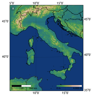
Figure 1:The domain the high-resolution fields cover: elevation over Italy and the Alpine ridge. Figure 1 of Tomasi et al. (2025), Geoscientific Model Development, CC BY 4.0.
Q1: Preprocessing the ERA5, COSMO-CLM and static datasets
Can you complete the code to preprocess the dataset for training the LDM?
Within the downloaded data_LDM folder, the file “preprocessing.py” (ldm_helpers/preprocessing.py) has been provided with helper functions so as to not clutter this notebook. Go ahead and inspect it for a better understanding of the steps used for preprocessing the dataset.
For a quick overview, here are the different functions present in the preprocessing file:
decompress_zst_pt : this function is used for decompressing the .zst format dataset for 2020 that is stored in data_LDM directory. The library we use for such files is called “zstandard”. The job of this function is to load the file, decompress it and return it as a PyTorch object
load_static_dif : This function returns a PyTorch tensor of static variables. we shall use this to process two single band static variables namely DEM and latitude.
load_land_cover : Land cover is composed of multiple bands, consisting of 16 land cover categories, hence this function is dedicated to processing the land cover raster.
collate_fn : This function is used for dataloader batching, meaning that it stacks up all variables as a batch. This is also the function where we “upsample” the ERA5 field to be at 2.2 km using bilinear interpolation for feeding into the UNet. As a result, all images (features and targets) will be at 672x576 resolution as a result, and inputs/outputs are concatenated. combined_input will as a result be of shape [batch, channels, 672,576] and high res output will be of shape [batch, 1, 672, 576]
load_and_normalise: Says what it does. Normalises the variables after loading the files for 2020. Further, calculates the train, val and test splits according to the specifications (here, train:test:val = 0.7:0.15:0.15)
get_file_list: This is a function which returns the paired high res and low res files as a tuple of shape (high_file_path, low_file_path, hour). Note that you can further reduce the size of the dataset with this function (HOW?)
Go ahead and run the below cell to import these functions into your notebook for the DownscalingDataset and DownscalingDataModule
# the preprocessing helpers sit next to this notebook in the repository; on a fresh
# runtime (Google Colab, say) fall back to the copy shipped inside the archive
helper_dir = "ldm_helpers" if os.path.isdir("ldm_helpers") else os.path.join(data_dir, "data_LDM")
sys.path.insert(0, helper_dir)

import preprocessing

# point the helpers at the downloaded data, wherever pooch put it: get_file_list() and
# load_and_normalise() read these two module attributes at call time
preprocessing.DATA_DIR = os.path.join(data_dir, "data_LDM") + os.sep
preprocessing.STATIC_DIR = os.path.join(preprocessing.DATA_DIR, "static_vars")
Import the helper functions for preprocessing from the preprocessing.py file
from preprocessing import load_and_normalise, decompress_zst_pt, get_file_listWe now see the implementation of the DownscalingDataset class in PyTorch, which determines how each sample is loaded (that is why it takes Dataset as the argument). This actually defines how to load a single sample with a batch containing channels with static and dynamical target (ground truth) and feature (input) fields.
Feel free to check out the preprocessing.py to get an idea of how the dataset was processed
class DownscalingDataset(Dataset):
    def __init__(self, file_list, static_vars, low_2mt_mean, low_2mt_std):
        self.file_list = file_list  # List of (high_file, low_file, date)
        self.static_vars = static_vars # for a list of static variables, refer the preprocessing file
        self.low_2mt_mean = _________
        self.low_2mt_std = __________
        self.samples = []


         # What is the temporal resoluton of our dataset?

        for hf, lf, date in self.file_list:
            for hour in range(24):
                self.samples.append((hf, ____, hour)) #returns a tuple of high_res,low_res and hour

    def __len__(self):
        return len(self.samples)

    def __getitem__(self, idx):
        hf, lf, hour = self.samples[idx]
        high_data = decompress_zst_pt(hf)
        low_data = decompress_zst_pt(___)
        high_t2m = high_data[hour]["2mT"].float().unsqueeze(0)  #[672, 576]
        low_t2m = low_data[hour]["2mT"].float().unsqueeze(0) #How much coarser are the coarse fields? What is the downscaling factor?
        #Can you print the dimensions of the high res and low res the dataset?
        #Can you figure out which variables we need?
        dem = self.static_vars["dem"].unsqueeze(0)
        lat = self.static_vars[_____].unsqueeze(0)
        lc = self.static_vars[_____]


        #How are the inputs upsampled ? and why?
        fuzzy_input = torch.cat([
            F.interpolate(low_t2m.unsqueeze(0), size=high_t2m.shape[-2:], mode='bilinear', align_corners=False).squeeze(0),
            dem, lat, lc
        ], dim=0)
        return fuzzy_input, _______
Just to assert the importance of above code cell, the above class will be used by the PyTorch Lightning DataLoader in due course to obtain samples during the train/val/test process.
Q2: What is PyTorch Lightning and how does it differ from PyTorch?
PyTorch Lightning is an elegant lightweight wrapper that removes the hassle of writing and rewriting boilerplate code by “wrapping” (duh) the standard code such as data splitting and training. This helps with scaling the code, reproducing the experiments and also clean the code up by avoiding repetitions. In a nutshell, you are still using PyTorch. Lightning just is your organisation buddy!
A great resource to learn about the differences between PyTorch and PyTorch Lightning and how PyTorch Lightning makes your life easier: https://
| PyTorch | PyTorch Lightning | |
|---|---|---|
| Training loop | Written out by hand, including moving data to the GPU, computing gradients and stepping the optimizer | Written once in the Trainer; you define hooks and callbacks instead |
| Model setup | Model, loss, optimizer and the rest are defined and wired up explicitly | Standardised methods on the LightningModule |
| GPU and distributed training | Devices and multi-GPU strategies are managed manually | Set by configuration; the number of devices is an argument |
| Logging and experiment tracking | Implemented by hand against TensorBoard or another logger | Built-in loggers (TensorBoard, CSV, WandB, Comet) |
| Checkpointing | Implemented by hand | ModelCheckpoint, out of the box |
| Code structure | Left to the author, so it varies between projects | Enforced by the LightningModule interface |
The trade-off is the usual one for a wrapper: less boilerplate and a structure other people can read, in exchange for having to learn where the library expects each piece of your code to go.
Now, for organising the process of loading the data, we use the PyTorch Lightning wrapper to wrap the previously coded DownscalingDataset class in a lightning friendly interface, the significance/handiness of which will be realised later. (short answer: it wraps dataloaders for the lightning TRAINER! wait for the long procedural answer which will be provided in due course ).
Just remember : while the DownscalingDataset class dictates how we load a single sample, the DownscalingDataModule below dictates the entire organisation, splitting of datasets and batchification for the entire pipeline !
Can you complete the code below for the DownscalingDataModule?
class DownscalingDataModule(LightningDataModule):
    def __init__(self, batch_size, val_frac, test_frac, num_workers, static_dir, save_stats_json):
        super().__init__()
        self.batch_size = ______
        self.val_frac = ________
        self.test_frac = _______
        self.________ = num_workers
        self.static_dir = ________
        self.________ = save_stats_json #Saving the standardisation stats in a .json file is a good idea, for use later (provided you are not standardising data on the fly!)


    def setup(self, stage=None):
        static_vars, stats = load_and_normalise(
            self.static_dir,
            val_frac=self.val_frac,
            ______=self.test_frac,
            save_stats_json=self.save_stats_json
        )
        file_list = get_file_list()
        dataset = DownscalingDataset(
            file_list, static_vars,
            low_2mt_mean=stats["low_2mt_mean"],
            low_2mt_std=stats[_______]
        )
        N = len(dataset)
        n_val = int(self.val_frac * N)
        n_test = int(self._____* ______)
        n_train = N - (_______+_____)
        self.train_set = torch.utils.data.Subset(dataset, range(0, n_train))
        self.val_set = torch.utils.data.Subset(dataset, range(n_train, n_train + n_val))
        self.______ = torch.utils.data.Subset(dataset, range(n_train + n_val, N))

    def train_dataloader(self):
        return DataLoader(self.train_set, batch_size=self.batch_size, shuffle=True, num_workers=self.num_workers)

    def val_dataloader(self):
        _______________________________________________________________________________________________________

    def test_dataloader(self):
        ______________________________________________________________________________________________________

    @property
    def test_dataset(self):
        return self.test_set.dataset
Please note that in the following sections, we will sequentially go through the code for the entire pipeline, culminating in running the said pipeline in a single line of code with the suitable configurations!
Q3: UNet for Deterministic (Mean) Prediction
Now we start with the “residual learning” model hierarchy, starting with training our deterministic UNet. For this, we need two complementary classes. 1) A UNet class which defines the architecture of a simple UNet for the prediction of high resolution 2m temperature field based and 2) Again,the PyTorch Lightning wrapper that wraps around this UNet class and adds all the logical steps of training the model.
class UNet(nn.Module):
    def __init__(self, in_channels, out_channels, channels, kernel_size):
        super().__init__()
        self.conv1 = nn.Conv2d(in_channels, channels[0], kernel_size, padding=1)
        self.conv2 = nn.Conv2d(channels[0], channels[1], _________, _______)
        self.final = nn.Conv2d(channels[1], out_channels, 1)


    def forward(self, x):
        h = F.relu(self.conv1(x))
        h = F.relu(self.conv2(h))
        output = self.final(h)
        return _________
Can you complete the code for the Lightning Module below and recognise how different it is from the aforementioned UNet class?
In case you are curious about what the configuration object “cfg” does, it contains the list of hyperparameters that are customisable from a YAML configuration file. For now, complete the code below. We promise it would become clearer as you progress through this notebook !
class UNetLitModule(LightningModule):
    def __init__(
        self,
        net: torch.nn.Module = None,
        lr: float = 1e-3,
        optimizer: dict = None,
        scheduler: dict = None,
        loss_fn: torch.nn.Module = None,
        in_channels: int = 19,
        out_channels: int = 1,
        channels: list = [32, 16],
        kernel_size: int = 3,
    ):
        super().__init__()
        self.save_hyperparameters(logger=False, ignore=['net', 'loss_fn'])


        self.net = net if net is not None else UNet(
            in_channels=in_channels,
            out_channels=out_channels,
            channels=____________,
            kernel_size=____________,
        )
        self.loss_fn = loss_fn if loss_fn is not None else nn.MSELoss()

        #By default, we train with the mean squared error loss (MSE loss), but you are free to experiment from the losses here : https://docs.pytorch.org/cppdocs/api/nn/loss.html

        self.lr = lr
        self.hparams.optimizer = optimizer
        self.hparams.scheduler = ____________

    def forward(self, x):
        return self.net(x)

    def model_step(self, batch):
        fuzzy_input, sharp_target = batch
        pred = self.forward(_________)
        loss = self.loss_fn(pred, sharp_target)
        return loss, ______

    def training_step(self, batch, batch_idx):
        loss, pred = self.model_step(batch)
        self.log("train/loss", loss, on_step=True, on_epoch=True, prog_bar=True)
        return loss

    def validation_step(self, batch, batch_idx):
        loss, pred = self.model_step(batch)
        self.log("val/loss", loss, on_step=False, on_epoch=True, prog_bar=True)
        return loss

    def test_step(self, batch, batch_idx):
        loss, pred = self.model_step(________)
        self.log("_______", loss, on_step=False, on_epoch=True, prog_bar=True)
        return loss

    def configure_optimizers(self):
        opt_cfg = self.hparams.get("optimizer", None)
        sch_cfg = self.hparams.get("scheduler", None)
        if opt_cfg and opt_cfg["type"] == "AdamW":
            optimizer = torch.optim.AdamW(
                self.parameters(),
                lr=opt_cfg.get("lr", self.lr),
                betas=tuple(opt_cfg.get("betas", (0.5, 0.9))),
                weight_decay=opt_cfg.get("weight_decay", 1e-3)
            )
        else:
            optimizer = torch.optim.Adam(
                self.parameters(),
                lr=opt_cfg.get("lr", self.lr) if opt_cfg else self.lr,
                weight_decay=opt_cfg.get("weight_decay", 1e-4) if opt_cfg else 1e-4
            )
        if sch_cfg and sch_cfg["type"] == "ReduceLROnPlateau":
            scheduler = torch.optim.lr_scheduler.ReduceLROnPlateau(
                optimizer,
                patience=sch_cfg.get("patience", 2),
                factor=sch_cfg.get("factor", 0.25)
            )
            return {
                "optimizer": optimizer,
                "lr_scheduler": {
                    "scheduler": scheduler,
                    "monitor": sch_cfg.get("monitor", "val/loss"),
                    "frequency": 1,
                },
            }
        else:
            return _________
Q4: “Residual Learning” and predictive distributions: multiple equally valid answers?
UNet, being a deterministic regression model, gives us the conditional mean of the distribution of possible high resolution samples conditioned on a low resolution input. Herein lies the problem with regression based point prediction: unless we use a distribution to sample from, we cannot generate new samples.
However, due to the stochastic nature of downscaling, all different possibilities within the conditional distribution are possible realities! For more on conditional generative models, refer to https://
For conducting residual latent diffusion, we need an autoencoder to “encode” the residual between UNet prediction and the ground truth into latent space, followed by denoising and “reconstructing”/decoding the residuals back to pixel space to add to the UNet prediction. This way, we add different samples of the residual to the UNet prediction to “sharpen” the UNet prediction.
We now turn to generative modeling section, where we will take you step by step to actually generate samples from a conditional distribution, key to generative modeling.
Q5: What is a Variational Autoencoder?
We define a Variational Autoencoder as an infinite mixture model which makes use of the identity
\begin{aligned} p_{\theta}(\mathbf{x}) = \int_{\mathbf{z}} p_{\theta}(\mathbf{x} \bigm | \mathbf{z})p_{\mathbf{z}}(\mathbf{z})d\mathbf{z} \end{aligned}
Hence a conditional VAE will make use of the identity to encode latent variable z independent of the inputs we are conditioning on,
\begin{aligned} p_{\theta}(\mathbf{y} \bigm | \mathbf{x}) = \int_{\mathbf{z}} p_{\theta}(\mathbf{y} \bigm | \mathbf{z}, \mathbf{x})p_{\mathbf{z}}(\mathbf{z})d\mathbf{z} \quad\quad \triangleleft \end{aligned}
In context of climate downscaling, the simplest explanation for a VAE is that it is an architecture that encodes and decodes samples to/from latent space from the pixel space. The main idea is that the latent variable z should be “encoding” information about the distributional target y which is independent of what the conditional mean has already given us! This encoding/decoding is probabilistic, because encoder maps the input (in this cases, residuals from the UNet as we discussed before) to a distribution (with parameters mean and log_var). The decoder then reconstructs the input from the latent vector back to the pixel space. For the purpose of our present use case, the VAE will be used for encoding residual samples into for the diffusion denoising process.
For making our VAE work, we need a loss function, which is a combination of two types of losses :
KL divergence loss : defined as kl_divergence in the notebook. Computes the Kullback-Leibler Divergence, which is a metric which measures how much the learned latent distribution is different from a standard normal distribution (in this case, as it is temperature). In essence, this pushes the encoder decoder model to produce realistic latents distributed like a standard normal, so it can generalise well. It is also known as relative entropy . For more, https://
towardsdatascience .com /understanding -kl -divergence -f3ddc8dff254/.
def kl_divergence(mean, log_var):  #mean and log var are parameters for a Gaussian for the latent variables
    kl = 0.5 * (log_var.exp() + mean.square() - 1.0 - log_var)
    return kl.mean()
Reconstruction loss : This can be any loss, although most commonly used are simply L1 or L2 norm, measuring the error between reconstructed outputs and encoded inputs
Can you think of what makes an autoencoder variational? Hint : Conventional autoencoders use one deterministic loss!!! :)
Notes on the reparameterisation trick: fundamental to the training of generative architectures in DL
In generative architectures such as the VAE, reconstruction of inputs does not happen exactly, but it is sampled and generated. In other words, it learns a probabilistic distribution, which it samples and decodes from. However, remember that for backpropagation, which is a cornerstone for gradient based optimisation, this sampling operation has to be expressed mathematically in a differentiable way. Herein lies the genius of the reparameterisation trick. Refer to the code cell below where the VAE class is defined
class VAE(nn.Module):
    def __init__(self, latent_dim=36, hidden_dim=128):
        super().__init__()
        self.encoder = nn.Sequential(
            nn.Conv2d(1, hidden_dim, 3, padding=1), nn.ReLU(),
            nn.AdaptiveAvgPool2d(1),
            nn.Flatten()
        )
        self.fc_mu = nn.Linear(hidden_dim, latent_dim)
        self.fc_logvar = nn.Linear(hidden_dim, latent_dim)
        self.fc_decode = nn.Linear(latent_dim, hidden_dim)
        self.decoder = nn.Sequential(
            nn.Unflatten(1, (hidden_dim, 1, 1)),
            nn.ConvTranspose2d(hidden_dim, 32, 8, stride=8),
            nn.ReLU(),
            nn.ConvTranspose2d(32, 1, 84, stride=84),
        )

    def encode(self, x):
        h = self.encoder(x)
        return self.fc_mu(h), self.fc_logvar(h)

    def reparameterize(self, mu, logvar):
        std = (0.5 * logvar).exp()
        return mu + std * torch.randn_like(std) #<---------------REPARAMETERISATION TRICK (explained below)!!!

    def decode(self, z):
        h = self.fc_decode(z)
        x = self.decoder(____)
        x = F.interpolate(x, size=(672, 576), mode='bilinear', align_corners=False)
        return ______

    def forward(self, x, sample_posterior=True):
        mu, logvar = self.encode(x)
        z = self.reparameterize(mu, logvar) if sample_posterior else mu
        recon = self.decode(z)
        return recon, mu, ______
So what did we do? Instead of sampling z (latent variable) deterministically, we rewrote the sampling step so that the gradients can now flow from the loss back to the encoder. (This explanation follows Understanding the reparameterization trick.)
In a nutshell, the reparameterisation trick allows backpropagation through a stochastic variable z. For a diagonal Gaussian:
where:
and are the encoder outputs for input (x)
is random noise sampled from a standard normal
Now, the noise (randomness) is contained in , and and are differentiable again!
Back to being hands on, we have to wrap the VAE class above in a PyTorch Lightning wrapper as we did with the UNet
class VAELitModule(LightningModule):
    def __init__(self, vae, unet_module, kl_weight=0.001, lr=1e-3):
        super().__init__()
        self.vae = vae
        self.unet = unet_module
        self.kl_weight = kl_weight
        self.lr = lr

    def training_step(self, batch, batch_idx):
        fuzzy_input, sharp_target = batch
        with torch.no_grad():
            unet_pred = self.unet(fuzzy_input)
        residual = sharp_target - unet_pred
        # Only use the UNet-predicted temperature channel as condition


        condition = unet_pred[:, 0:1]
        recon, mu, logvar = self.vae(_________) #encode residuals into latent space

        recon_loss = F.mse_loss(recon, residual)
        kl_loss = kl_divergence(mu, logvar)
        total_loss = recon_loss + self.kl_weight * kl_loss
        self.log("train/loss", total_loss)
        return total_loss

    def validation_step(self, batch, batch_idx):
        fuzzy_input, sharp_target = batch
        with torch.no_grad():
            unet_pred = self.unet(_________)
        residual = sharp_target - unet_pred
        condition = unet_pred[:, 0:1]
        recon, mu, logvar = self.vae(________) #encode residuals into latent space
        recon_loss = F.mse_loss(recon, _________)
        kl_loss = kl_divergence(mu, logvar)

        #What are the different components of the total VAE loss?

        total_loss = __________ + self.kl_weight * kl_loss
        self.log("val/loss", total_loss)
        return total_loss

    def configure_optimizers(self):
        return torch.optim.Adam(self.parameters(), lr=self.lr)
Q6: Denoising UNet for the latent space (Latent Diffusion)
Now that we have the encoded residuals in latent space, we can “denoise” these latent vectors using a UNet backbone for generating residual samples in the latent space, and then decode them back to pixel space to add to the original UNet mean prediction to generate samples of high resolution images conditioned on the coarse ERA5 + static predictors.
In the below LatentDenoiser class, we have coded a neural network that predicts the noise that is added to latent vectors at each diffusion timestep. The VAE is frozen during training the denoiser.
class LatentDenoiser(________):
    def __init__(self, in_channels, out_channels, channels, kernel_size, context_channels=0):
        super().__init__()
        self.time_embed = nn.Sequential(
            nn.Linear(1, channels[0]),
            nn.ReLU(),
            nn.Linear(channels[0], channels[0])
        )
        self.unet = UNet(
            in_channels=in_channels + 2 + context_channels,  # +context_channels
            out_channels=out_channels,
            channels=channels,
            kernel_size=kernel_size
        )


    def forward(self, z_noisy, unet_pred, timestep=None, context=None):
        if timestep is None:
            timestep = torch.zeros(z_noisy.shape[0], 1, device=z_noisy.device)
        if timestep.dim()==1:
            timestep = timestep.unsqueeze(1)

        B, _, H, W = z_noisy.shape
        t_embed = self.time_embed(timestep.float())
        t_map = t_embed[:, :1].unsqueeze(-1).unsqueeze(-1).expand(-1, 1, H, W)
        inputs = [z_noisy, unet_pred, t_map]
        if context is not None:
            inputs.append(context)
        x = torch.cat(inputs, dim=1)
        return self.unet(________)
For the Lightning Module of the LDM, following are the steps:
The UNet prediction as well as the VAE are frozen, so that the encoded residuals are denoised in latent space by the UNet
The denoising UNet LatentDenoiser() class above is instantiated, that predicts noise in the latent space
register_noise_schedule creates a schedule of noise levels (how much noise will be added at each step) for each timestep in the process of diffusion
The q_sample method adds noise to a latent at a given timestep t using the schedule prescribed above. It is used to simulate the diffusion forward by corrupting the latent gradually
p_losses samples a noisy latent vector at t and denoiser predicts the noise that was added at t . It then computes losses between predicted noise and the true noise level according to schedule
sample : starts from completely random latent space noise and then performs iterative denoising using UNet denoiser and reverse diffusion. The final denoised latent is returned.
generate_samples : samples new latents using the diffusion process and finally decodes them back to pixel space as images of residuals to be added to UNet.
class LDMLitModule(LightningModule):
    def __init__(
        self,vae,latent_dim=36,conditioner=None,latent_height=6,latent_width=6,lr=1e-4,num_timesteps=50,
        noise_schedule="linear", #Alternative?
        loss_type="l2",hidden_dim=128,num_layers=4,
        param_type="eps", #Alternative?
        optimizer=None,scheduler=None,
    ):
        super().__init__()

        assert latent_dim == latent_height * latent_width, (
            f"latent_dim ({latent_dim}) must be equal to "
            f"latent_height*latent_width ({latent_height}*{latent_width})"
        )

        if param_type not in {"eps", "x0", "v"}:
            raise ValueError(f"Unknown param_type: {param_type}")

        self.save_hyperparameters(logger=False, ignore=["vae"])


        self.vae = vae.vae.requires_grad_(False)
        self.vae.eval()

        self.unet = vae.unet.requires_grad_(False)
        self.unet.eval()

        self.conditioner = ____________
        self.latent_height = ___________
        self.latent_width = ___________
        self.lr = __________
        self.num_timesteps = ____________
        self.param_type = param_type

        self.denoiser = LatentDenoiser(in_channels=1,out_channels=1,channels=[hidden_dim] * num_layers,kernel_size=3,
            context_channels=1,
        )

        self.loss_fn = {
            "______": nn.L1Loss(),
            "______": nn.MSELoss(),
        }[loss_type]

        self.register_noise_schedule(noise_schedule)

        self.hparams.optimizer = ___________
        self.hparams.scheduler = ___________


    def register_noise_schedule(self, schedule="linear"):


        if schedule == "linear":
            betas = torch.linspace(
                1e-4,
                2e-2,
                self.num_timesteps,
                dtype=torch.float32,
            )

        elif schedule == "cosine":
            steps = torch.arange(
                self.num_timesteps + 1,
                dtype=torch.float32,
            )

            s = 0.008
            x = (steps / self.num_timesteps + s) / (1 + s)
            alpha_bar = torch.cos(x * torch.pi / 2).square()
            alpha_bar = alpha_bar / alpha_bar[0]

            betas = 1.0 - alpha_bar[1:] / alpha_bar[:-1]
            betas = betas.clamp(1e-5, 0.999)

        else:
            raise ValueError(f"Unknown schedule: {schedule}") #Please go ahead and read about other noise schedules

        alphas = 1.0 - betas
        alphas_cumprod = torch.cumprod(alphas, dim=0)
        alphas_cumprod_prev = F.pad(
            alphas_cumprod[:-1],
            (1, 0),
            value=1.0,
        )

        posterior_variance = (
            betas
            * (1.0 - alphas_cumprod_prev)
            / (1.0 - alphas_cumprod)
        )

        self.register_buffer("betas", _________)
        self.register_buffer("alphas", __________)
        self.register_buffer("alphas_cumprod", ___________)


        self.register_buffer(
            "sqrt_alphas_cumprod",
            torch.sqrt(___________),
        )
        self.register_buffer(
            "sqrt_one_minus_alphas_cumprod",
            torch.sqrt(_______ - alphas_cumprod),
        )
        self.register_buffer(
            "sqrt_recip_alphas",
            torch.sqrt(1.0 / alphas),
        )
        self.register_buffer(
            "posterior_variance",
            posterior_variance.clamp(min=1e-20),
        )


##############################################


    def q_sample(self, x_start, t, noise=None):
        """
        Forward diffusion:
        """
        if noise is None:
            noise = torch.randn_like(__________) #Hint: The latent has to match in shape with the starting latent vector

        sqrt_alpha_bar = self.sqrt_alphas_cumprod[t].view(
            -1, 1, 1, 1
        )
        sqrt_one_minus_alpha_bar = (
            self.sqrt_one_minus_alphas_cumprod[t]
            .view(-1, 1, 1, 1)
        )

        return (
            sqrt_alpha_bar * x_start
            + sqrt_one_minus_alpha_bar * noise
        )


####################################################


    def _prediction_to_eps(self, model_output, x_t, t):
        alpha = self.sqrt_alphas_cumprod[t].view(-1, 1, 1, 1)
        sigma = self.sqrt_one_minus_alphas_cumprod[t].view(
            -1, 1, 1, 1
        )

        if self.param_type == "eps": #What does this predict?
            return model_output

        if self.param_type == "x0": #What does this predict?
            return (
                x_t - alpha * model_output
            ) / sigma.clamp_min(1e-5)

        if self.param_type == "v": #What does this predict?
            return sigma * x_t + alpha * model_output

        raise ValueError(
            f"Unknown param_type: {self.param_type}"
        )


    ############################################################


    @torch.no_grad()
    def sample(self,latent_shape,unet_pred_ds,context=None,device=None):

        if device is None:
            device = next(self.parameters()).device

        z = torch.randn(latent_shape, device=device) #what is the shape of this latent vector?
        unet_pred_ds = unet_pred_ds.to(device)

        if context is not None:
            context = context.to(device)

        for timestep in reversed(range(self.num_timesteps)):
            t = torch.full(
                (z.shape[0],),
                timestep,
                dtype=torch.long,
                device=device,
            )

            model_output = self.denoiser(
                z,
                unet_pred_ds,
                t,
                context=context,
            )

            eps_pred = self._prediction_to_eps(
                model_output,
                z,
                t,
            )

            beta_t = self.betas[timestep]
            sqrt_recip_alpha_t = self.sqrt_recip_alphas[timestep]
            sqrt_one_minus_alpha_bar_t = (
                self.sqrt_one_minus_alphas_cumprod[timestep]
            )

            mean = sqrt_recip_alpha_t * (
                z
                - beta_t
                / sqrt_one_minus_alpha_bar_t
                * eps_pred
            )

            if timestep > 0: #What happens at the last timestep in this reverse diffusion process?

                noise = torch.randn_like(z)
                z = mean + torch.sqrt(
                    self.posterior_variance[timestep]
                ) * noise
            else:
                z = mean

        return z

    ###################################################

    def p_losses(
        self,x_start,unet_pred,t,noise=None,context=None,
    ):
        if noise is None:
            noise = torch.randn_like(___________)

        x_noisy = self.q_sample(___________, t, noise)

        batch_size = x_noisy.shape[0]
        x_noisy = x_noisy.view(
            batch_size,
            1,
            self.latent_height,
            self.latent_width,
        )

        unet_pred_ds = F.interpolate(
            unet_pred,
            size=(self.latent_height, self.latent_width),
            mode="bilinear",
            align_corners=False,
        ) #To ensure the UNet prediction has the same spatial dimensions as the latent representation, not necessary if you have checked the shapes beforehand!

        context_ds = None

        if self.conditioner is not None and context is not None:
            context_ds = self.conditioner(context)

        predicted = self.denoiser(
            x_noisy,
            unet_pred_ds,
            t,
            context=__________,
        )

        noise_4d = noise.view_as(x_noisy)

        x_start_4d = x_start.view_as(x_noisy)

        if self.param_type == "eps":
            target = noise_4d

        elif self.param_type == "_______":
            target = x_start_4d

        else:
            alpha_t = self.sqrt_alphas_cumprod[t].view(
                -1, 1, 1, 1
            )
            sigma_t = self.sqrt_one_minus_alphas_cumprod[t].view(
                -1, 1, 1, 1
            )
            target = alpha_t * noise_4d - sigma_t * x_start_4d

        return self.loss_fn(predicted, target)


    ###################################################

    def forward(self,fuzzy_input,unet_pred,sharp_target,context=None,
    ):
        del fuzzy_input

        with torch.no_grad():
            residual = sharp_target - unet_pred
            mu, logvar = self.vae.encode(__________)
            z = self.vae.reparameterize(mu, _______)

        expected_latent_dim = self.latent_height * self.latent_width


        #Check the shapes here , especially before reshaping z into the latent spatial dimensions.

        print(f"Residual shape: {_____________}")
        print(f"Mu shape: {__________}, Logvar shape: {___________}")


        assert z.shape[1] == expected_latent_dim, (
            f"Latent shape mismatch: got {z.shape}; "
            f"expected latent dimension {expected_latent_dim}"
        )

        z = z.view(
            z.shape[0],
            1,
            self.latent_height,
            self.latent_width,
        )

        t = torch.randint(
            0,
            self.num_timesteps,
            (z.shape[0],),
            device=z.device,
        )


        return self.p_losses(
            z,
            unet_pred,
            t,
            context=context,
        )

    def _shared_step(self, batch):
        fuzzy_input, sharp_target = batch

        with torch.no_grad():
            unet_pred = self.unet(fuzzy_input)

        context = unet_pred[:, 0:1] #Can you think of a richer context representation?

        return self(
            fuzzy_input,
            ____________,
            sharp_target,
            context=_________,
        )

    ##################################


    def training_step(self, batch, batch_idx):
        loss = self._shared_step(batch)

        self.log(
            "train/loss",
            loss,
            on_step=True,
            on_epoch=True,
            prog_bar=True,
            sync_dist=True,
        )

        return loss


    ###################################

    def validation_step(self, batch, batch_idx):
        loss = self._shared_step(batch)

        self.log(
            "val/loss",
            loss,
            on_step=False,
            on_epoch=True,
            prog_bar=True,
            sync_dist=True,
        )

        return loss

    ####################################


    def test_step(self, batch, batch_idx):
        loss = self._shared_step(batch)

        self.log(
            "test/loss",
            loss,
            on_step=False,
            on_epoch=True,
            prog_bar=True,
            sync_dist=True,
        )

        return ________

#############################################

    def configure_optimizers(self):
        opt_cfg = self.hparams.get("optimizer")
        sch_cfg = self.hparams.get("scheduler")

        trainable_params = [
            parameter
            for parameter in self.parameters()
            if parameter.requires_grad
        ]

        if opt_cfg and opt_cfg.get("type") == "AdamW":
            optimizer = torch.optim.AdamW(
                trainable_params,
                lr=opt_cfg.get("lr", self.lr),
                betas=tuple(
                    opt_cfg.get("betas", (0.5, 0.9))
                ),
                weight_decay=opt_cfg.get(
                    "weight_decay",
                    1e-3,
                ),
            )
        else:
            optimizer = torch.optim.Adam(
                trainable_params,
                lr=opt_cfg.get("lr", self.lr)
                if opt_cfg
                else self.lr,
                weight_decay=opt_cfg.get(
                    "weight_decay",
                    1e-4,
                )
                if opt_cfg
                else 1e-4,
            )

        if (
            sch_cfg
            and sch_cfg.get("type") == "ReduceLROnPlateau"
        ):
            scheduler = torch.optim.lr_scheduler.ReduceLROnPlateau(
                optimizer,
                patience=sch_cfg.get("patience", 5),
                factor=sch_cfg.get("factor", 0.5),
            )

            return {
                "optimizer": optimizer,
                "lr_scheduler": {
                    "scheduler": scheduler,
                    "monitor": sch_cfg.get(
                        "monitor",
                        "val/loss",
                    ),
                    "frequency": 1,
                },
            }

        return ______________
In the above LatentDenoiser class and LightningModule, we have coded a neural network that predicts the noise that is added to latent vectors at each diffusion timestep. The VAE is frozen during training the denoiser. The noise schedule (which can be either linear or cosine) controls how noise is added at each timestep. The module, in essence, learns to then generate or denoise latent representations using a diffusion process, making it possible to sample new, realistic data from the latent vectors back to pixel space.
In the original paper and repository, the authors condition on a range of variables to provide more context to the model, using AFNO (Attention Fourier Neural Operator) attention blocks. For the sake of simplicity, we use a simple CNN to downsample the UNet prediction and use it as “context” tensor, to be concatenated to the latent variable z. Simply put, the conditioner class is a simple neural network for providing conditional information to the denoising process during diffusion. It serves the purpose of processing context data, eg., outputs a feature map that matches the latent space dimensions
#for conditional generation:: a conditioner class

#Can you compare this simple conditioner class with the AFNO class laid out in the source paper?

class Conditioner(____________):
    def __init__(self, in_channels, out_channels, latent_height, ________):
        super().__init__()
        self.net = nn.Sequential(
            nn.Conv2d(in_channels, 32, 3, padding=1),
            nn.ReLU(),
            nn.Conv2d(32, out_channels, 3, padding=1),
            nn.AdaptiveAvgPool2d((latent_height, latent_width))
        )


    def forward(self, x):
        return self.net(______)
Q7: Training the entire LDM_res hierarchy using a configuration file (YAML)
We have come a long way with extensive amount of code. So in case you wish to conduct sensitivity experiments and hyperparameter optimisation, do you have to make granular changes in each section of this tedious codebase? In case we need to change anything, do we really go back through the entire model and change every single thing we want to change?
The answer is NO! That is why we used PyTorch Lightning :) Now that we have the UNet, VAE and LDM classes along with their respective Lightning Modules, we are ready to train the entire hierarchy using a single configuration file (YAML) with our choice of hyperparameters. YAML is a data serialisation that is human readable and can be used to generate configuration files for conducting a range of experiments without changing the source code. For a primer on YAML : https://
First, go ahead and complete the training hierarchy function defined below. Then we shall write a YAML file to conduct experiments with the trained models. In case these seem to be a lot of steps, please do not be overwhelmed. Go through the code step by step to understand (and make sure to use a GPU!):
We split our low res high res pairs into training, validation and testing
Then we train the UNet to predict the conditional mean of the high resolution output.
To further sharpen the image that is the UNet prediction, we calculate the residuals (difference between UNet prediction and the ground truth) and encode it into latent space using the encoder of the VAE
Next, we “denoise” these residuals in latent space using the denoising UNet
The “decoder” of the trained VAE decodes (reconstructs) the image back to pixel space (these are residuals)
Please note that in the interest of time, we have already trained and placed some model checkpoints in the data_LDM/checkpoints directory. In any case, the train_hierarchy() function makes sure that you have both options : training your own models (if your memory and compute allow) as well as also load pretrained weights to have fun with visualisation and analysis!
#Monkey patching for torch.load to always set weights_only=False

#In case you get a recursion-related error in this cell, please restart your kernel and run the notebook from end to end.

_orig_load = torch.load
def _patched_load(*args, **kwargs):
    kwargs["weights_only"] = False
    return _orig_load(*args, **kwargs)
torch.load = _patched_load
def train_hierarchy(cfg):
data_module = DownscalingDataModule(
batch_size=cfg.data.batch_size,
val_frac=cfg.data.val_split,
test_frac=_____________,
num_workers=______________,
static_dir=_______________,
save_stats_json=os.path.join(cfg.paths.output_dir, "stats.json")
#stats.json was saved when you preprocessed the dataset! The path should be data_LDM/stats.json
)
data_module.setup()
#Selecting/Making checkpoint directories for UNet, VAE, and LDM
# (data_LDM/checkpoints currently points to the pretrained models)
checkpoint_dir = cfg.paths.checkpoint_dir
os.makedirs(checkpoint_dir, exist_ok=True)
unet_ckpt_dir = os.path.join(checkpoint_dir, "unet")
os.makedirs(unet_ckpt_dir, exist_ok=True)
unet_ckpts = sorted([f for f in os.listdir(unet_ckpt_dir) if f.endswith(".ckpt")])
if unet_ckpts:
#If a pretrained UNet checkpoint exists, this code block loads it.
#Change the checkpoint dir to train your own model
print("Loading pretrained UNet ckpt")
unet_module = UNetLitModule.load_from_checkpoint(os.path.join(unet_ckpt_dir, unet_ckpts[-1]))
else:
print("Training UNet")
unet_module = ___________(
net=UNet(
in_channels=cfg.model.unet.in_channels,
out_channels=cfg.model.unet.out_channels,
channels=cfg.model.unet.channels,
kernel_size=cfg.model.unet.kernel_size,
),
lr=cfg.model.unet.lr,
optimizer=cfg.optimizer.unet,
scheduler=cfg.scheduler.unet,
)
unet_checkpoint = ModelCheckpoint(
dirpath=unet_ckpt_dir,
filename="unet-{epoch:02d}",
save_top_k=1,
monitor="val/loss",
mode="min",
)
trainer_unet = Trainer(
max_epochs=cfg.training.unet_epochs,
accelerator=cfg.trainer.accelerator,
gradient_clip_val=cfg.trainer.get("gradient_clip_val", 1.0),
enable_checkpointing=True,
logger=False,
callbacks=[unet_checkpoint],
)
___________.fit(unet_module, datamodule=data_module)
vae_ckpt_dir = os.path.join(checkpoint_dir, "vae")
os.makedirs(vae_ckpt_dir, exist_ok=True)
vae_ckpts = sorted([f for f in os.listdir(vae_ckpt_dir) if f.endswith(".ckpt")])
if vae_ckpts:
print("Loading pretrained VAE ckpt")
vae = ________(latent_dim=cfg.model.vae.latent_dim,hidden_dim=cfg.model.vae.hidden_dim
)
vae_module = ___________.load_from_checkpoint(
os.path.join(vae_ckpt_dir, vae_ckpts[-1]),
vae=vae,
unet_module=unet_module
)
else:
print("Training VAE")
vae = VAE(
latent_dim=cfg.model.vae.latent_dim,
hidden_dim=cfg.model.vae.hidden_dim
)
vae_module = VAELitModule(
vae=vae,
unet_module=unet_module,
kl_weight=cfg.model.vae.kl_weight,
lr=cfg.model.vae.lr
)
vae_checkpoint = _______________(
dirpath=vae_ckpt_dir,
filename="vae-{epoch:02d}",
save_top_k=1,
monitor="val/loss",
mode="min",
)
trainer_vae = _____________(
max_epochs=cfg.training.vae_epochs,
accelerator=cfg.trainer.accelerator,
enable_checkpointing=True,
logger=False,
default_root_dir=vae_ckpt_dir,
callbacks=[vae_checkpoint],
)
____________.fit(vae_module, datamodule=data_module)
ldm_ckpt_dir = os.path.join(checkpoint_dir, "ldm")
os.makedirs(ldm_ckpt_dir, exist_ok=True)
ldm_ckpts = sorted([f for f in os.listdir(ldm_ckpt_dir) if f.endswith(".ckpt")])
if ldm_ckpts:
print("Loading pretrained LDM ckpt")
ldm_module = LDMLitModule.load_from_checkpoint(os.path.join(ldm_ckpt_dir, ldm_ckpts[-1]),
vae=vae_module,
strict=False,
)
else:
print("Training LDM")
conditioner= ___________(
in_channels= 1,
out_channels= 1,
latent_height=cfg.model.ldm.latent_height,
latent_width=cfg.model.ldm.latent_width
)
ldm_module = LDMLitModule(
vae=vae_module,
conditioner=__________,
latent_dim=cfg.model.ldm._________,
latent_height=_____________________,
latent_width=cfg.model.ldm.latent_width,
lr=cfg.model.ldm.lr,
num_timesteps=___________________,
noise_schedule=cfg.model.ldm.noise_schedule,
loss_type=cfg.model.ldm.loss_type,
____________=cfg.model.ldm.hidden_dim,
_____________=cfg.model.ldm.num_layers,
_____________=cfg.optimizer.ldm,
scheduler=cfg.scheduler.ldm,
param_type=______________,
)
ldm_checkpoint = ModelCheckpoint(
dirpath=ldm_ckpt_dir,
filename="ldm-{epoch:02d}",
save_top_k=1,
monitor="val/loss",
mode="min",
)
trainer_ldm = Trainer(
max_epochs=cfg.training.ldm_epochs,
accelerator=cfg.trainer.accelerator,
enable_checkpointing=True,
logger=False,
default_root_dir=ldm_ckpt_dir,
callbacks=[ldm_checkpoint],
)
trainer_ldm.fit(ldm_module, datamodule=data_module)For your first experiment with the above training hierarchy function, go ahead and write your first YAML configuration file. In case you do not specify anything, the default setting in the source code is used by the model. Feel free to play with different configurations! Below is the config file using which we have trained the pretrained models provided in data_LDM/checkpoints. Please note that you can train your own models and save them IN A SEPARATE DIRECTORY.
YAML files can be created using the template below (only an example!)
cfg_dict = {
    "data": {
        "batch_size": 32,
        "num_workers": 1,
        "test_split": 0.15,
        "val_split": 0.15,
    },
    "model": {
        "ldm": {
            "hidden_dim": 64,
            "latent_height": 6,
            "latent_width": 6,
            "latent_dim": 36,
            "loss_type": "l2",
            "lr": 0.0001,
            "noise_schedule": "linear",
            "num_layers": 2,
            "num_timesteps": 20,
            "param_type": "eps",
        },
        "unet": {
            "channels": [32, 16],
            "in_channels": 19,
            "kernel_size": 3,
            "lr": 0.0001,
            "out_channels": 1,
        },
        "vae": {
            "decoder_channels": [8],
            "encoder_channels": [8],
            "hidden_dim": 128,
            "input_channels": 2,
            "input_height": 672,
            "input_width": 576,
            "kl_weight": 0.001,
            "latent_dim": 36,
            "lr": 0.0001,
        },
    },
    "optimizer": {
        "ldm": {
            "betas": [0.5, 0.9],
            "lr": 0.0001,
            "type": "AdamW",
            "weight_decay": 0.001,
        },
        "unet": {
            "lr": 0.0001,
            "type": "Adam",
            "weight_decay": 0.0001,
        },
        "vae": {
            ______: [0.5, 0.9],
            _______: 0.0001,
            _______: "AdamW",
           ________: 0.001,
        },
    },
    "paths": {
        "checkpoint_dir": f"{data_dir}/data_LDM/checkpoints", #Remember to change this for avoiding overwriting the pretrained models with your own models !!
        "data_dir": f"{data_dir}/data_LDM",
        "output_dir": "./",
        "static_dir": f"{data_dir}/data_LDM/static_vars",
    },
    "scheduler": {
        "ldm": {
            "factor": 0.25,
            "monitor": "val/loss",
            "patience": 3,
            "type": "ReduceLROnPlateau",
        },
        "unet": {
            "factor": 0.25,
            "monitor": "val/loss",
            "patience": 3,
            "type": "ReduceLROnPlateau",
        },
        "vae": {
            "factor": 0.25,
            "monitor": "val/recon_loss",
            "patience": 3,
            "type": "ReduceLROnPlateau",
        },
    },
    "seed": 42,
    "trainer": {
        "accelerator": "gpu",
        "gradient_clip_val": 1.0,
        "max_epochs": 10,
        "min_delta": 0.0001,
    },
    "training": {
        "ldm_epochs": 20,
        "unet_epochs": 20,
        "vae_epochs": 20,
    },
}
We convert the above code block into a YAML config file as
cfg = OmegaConf.create(cfg_dict)
OmegaConf.save(cfg, "config_experiments.yaml")
You should now see the configuration file in your present working directory. Open it and inspect whether it is the same as what we wrote above!
Create this .yaml file and load it later in the cfg variable (as that is how it is referred to in the source code for all the PyTorch and Lightning wrappers). Now you know what the object “cfg” is in all the LightningModules in this notebook!Can you go back and inspect in what places we have used cfg objects? Does this explain the purpose of using config objects alongside default values modularised code and easy experimentation?
with open("config_experiments.yaml", "w") as f:
    yaml.dump(cfg_dict, f, default_flow_style=False)
From now on, it should be clear that PyTorch Lightning in conjunction with a configuration manager such as OmegaConf or Hydra (built on OmegaConf, with even more advanced functionalities for configuring experiments) are indispensable for performing and logging experiments. We have barely scratched the surface of their functionalities in this notebook! For a primer on OmegaConf and Hydra: https://
For the purposes of running this pipeline, we stick to OmegaConf
cfg = OmegaConf.load("______________")
train_hierarchy(cfg) #Make sure to run this on a GPU!!!
You can see that the UNet and VAE are being loaded from a pretrained checkpoint. This is for saving time ! As the entire hierarchy of sequential models will take very long to train (approx 45 minutes from our experience of training it), we have ensured that you have pretrained models at your disposal. But feel free to try training them on your own (do not forget to change the checkpoint directory to avoid overwriting pretrained models!). See if you can train and compare configurations of your own.
Q8: Inference pipeline for visualising a single frame and generated samples
Fill out the code cell below to load the three pretrained architectures, and visualising a single frame from coarse input all the way to high resolution samples .
The below code:
Loads standardisation stats from the .json file saved before
Initialises the data module and loads the test set
Loads the checkpointed models (UNet, VAE and LDM) and sets all models to eval mode
Selects a random test frame for inference and prepares as input for the pixel UNet
Runs the frame through the hierarchy (UNet, encoding of residuals, VAE, LDM and decoding)
Samples three samples (latent vectors) from VAE, decodes them to generate three possible residuals, and adds these to the UNet to predict three different reconstructions
Finally destandardises all outputs for visualising the frames and plots the six images : ground truth, ERA5 input field, UNet prediction, three generated samples
Start by setting up the test dataloader:
data_module = ______________(
    batch_size=1,
    val_frac=cfg.data.val_split,
    test_frac=cfg.data.test_split,
    num_workers=cfg.data.num_workers, #try reducing number of workers if you encounter issues, even=0
    static_dir=cfg.paths.static_dir,
    save_stats_json=os.path.join(cfg.paths.output_dir, "stats.json")
)
data_module.setup()


____________ = data_module.test_dataloader()

# Get a single test sample (input and ground truth)

test_iter = iter(test_loader)
input_sample, ground_truth = next(test_iter)


input_sample = ____________
ground_truth = ground_truth[0]
The below inference_random_frame() function now takes in an input sample from ERA5 test set, feeds it into the model hierarchy, and generates 3 samples. All samples are then plotted against ground truth.
def inference_random_frame(cfg, input_sample, ground_truth=ground_truth, return_array=False):


    stats_path = os.path.join(cfg.paths.output_dir, "stats.json")
    with open(stats_path, "r") as f:
        stats = json.load(f)
    low_2mt_mean = stats["low_2mt_mean"]
    low_2mt_std = stats["low_2mt_std"]

    def denormalise(arr):
        return arr * low_2mt_std + low_2mt_mean

    # Loading models
    unet_ckpt_dir = os.path.join(cfg.paths.checkpoint_dir, "unet")
    unet_ckpt = sorted(os.listdir(unet_ckpt_dir))[-1]
    unet_module = UNetLitModule.load_from_checkpoint(os.path.join(unet_ckpt_dir, unet_ckpt))

    vae_ckpt_dir = os.path.join(cfg.paths.checkpoint_dir, "_________")
    vae_ckpt = sorted(os.listdir(_____________))[-1]
    vae = VAE(latent_dim=cfg.model.vae.latent_dim, hidden_dim=cfg.model.vae.hidden_dim)
    vae_module = VAELitModule.load_from_checkpoint(os.path.join(vae_ckpt_dir, vae_ckpt), vae=vae, unet_module=___________)


    ldm_ckpt_dir = os.path.join(_______________, "____________")
    ldm_ckpt = sorted(os.listdir(____________))[-1]

    conditioner = Conditioner(
        in_channels=1,
        out_channels=1,
        latent_height=cfg.model.ldm.latent_height,
        latent_width=cfg.model.ldm.latent_width,
    )

    ldm_module = LDMLitModule.load_from_checkpoint(
        os.path.join(ldm_ckpt_dir, ldm_ckpt),
        vae=vae_module,
        conditioner=_________,
        strict=False,
    )

    unet_module.eval()
    ________________()
    ________________()

    conditioner = ldm_module.conditioner
    ________________()


#Inference on a single frame

    with torch.no_grad():
        device = next(unet_module.parameters()).device
        ___________ = input_sample.unsqueeze(0).to(device)  # [1, C, H, W]
        unet_pred = unet_module.net(fuzzy_input)            # [1, 1, H, W]

        unet_pred_np= unet_pred[0, 0].cpu().numpy()

        latent_height = cfg.model.ldm.latent_height
        ____________ = cfg.model.ldm.latent_width
        ____________ = (1, 1, latent_height, latent_width)

        unet_pred_ds = F.interpolate(unet_pred, size=(___________, ____________), mode='bilinear', align_corners=False)
        context_tensor = conditioner(unet_pred_ds)  # [1, 1, latent_height, latent_width]

            # Generate 3 samples
        final_reconstructions = []


        for _ in range(3):
            z_sample = ldm_module.sample(latent_shape, unet_pred_ds, context=context_tensor)
            _____________ = z_sample.view(z_sample.size(0), -1)
            generated_residual = vae_module.vae.decode(z_sample_flat)
            final_reconstruction = unet_pred + ________________
            final_reconstructions.append(final_reconstruction[0, 0].cpu().numpy())


    if return_array:
        return np.stack(final_reconstructions, axis=0),unet_pred_np #Stacking a set of 3 predictions


    all_imgs = [
        denormalise(fuzzy_input[0, 0].cpu().numpy()),  # ERA5 predictor
        denormalise(unet_pred_np),                     # UNet prediction
        *[denormalise(img) for img in final_reconstructions],  # 3 samples
    ]


    titles = [
        "ERA5 2m input",
        "UNet Prediction",
        "Sample 1",
        "Sample 2",
        "Sample 3",

    ]

    if ground_truth is not None:
        all_imgs.append(denormalise(ground_truth.cpu().numpy().squeeze()))
        titles.append("Ground Truth")


    vmin = min(img.min() for img in all_imgs)
    vmax = max(img.max() for img in all_imgs)

    fig, axes = plt.subplots(1, len(all_imgs), figsize=(6 * len(all_imgs), 6), constrained_layout=True)


    images = []

    for i, ax in enumerate(axes):
        im = ax.imshow(all_imgs[i], cmap='coolwarm', vmin=vmin, vmax=vmax, origin='upper')
        ax.set_title(titles[i], fontsize=15, fontweight='bold')
        ax.set_xlabel("Longitude", fontsize=13)
        ax.set_ylabel("Latitude", fontsize=13)
        ax.tick_params(axis='both', which='major', labelsize=11)
        ax.grid(False, which='both')
        images.append(im)

    cbar = fig.colorbar(images[0], ax=axes, orientation='horizontal', fraction=0.04, pad=0.08)
    cbar.set_label("2m Temperature (degrees C)", fontsize=15, fontweight='bold')
    cbar.ax.tick_params(labelsize=13)

    plt.suptitle("ERA5 low res + 3 samples + Ground Truth", fontsize=20, y=1.05, fontweight='bold')
    plt.show()
To run the above inference pipeline, just run the below cell with the previously created configuration file!
inference_random_frame(________, input_sample, ground_truth=ground_truth)Q9: Can you establish the added value of generative downscaling?
No matter how wonderful and close to the ground truth (target) your frame looks, we have to quantify the overall added value of UNet and the VAE+LDM over simple bilinear interpolation to truly gauge whether all these lines of code were worth the effort! As you have already seen the CRPS score in previous notebooks, let us go ahead and calculate it (Using crps from the properscoring library https://
from properscoring import crps_ensembleall_crps_ldm = []
all_crps_era5 = []
__________ = []Now we write the loop to generate 3 samples for each frame in the test set
for input_sample, ground_truth in data_module.test_dataloader():


#Take care of the following : the crps_ensemble() function takes channels last, many times tensors have channel first
    # input_sample: (batch, C, H, W) or (batch, H, W)
    # ground_truth: (batch, 1, H, W) or (batch, H, W)

    for i in range(input_sample.shape[0]):

        inp = input_sample[i][0].cpu().numpy().squeeze()

        gt = ground_truth[i][0].cpu().numpy().squeeze()


        samples, unet_pred = inference_random_frame(cfg, input_sample[i], ground_truth=None, return_array=True)
        samples = np.moveaxis(samples, 0, -1)

        crps_ldm = crps_ensemble(gt, samples)
        all_crps_ldm.append(np.mean(crps_ldm))

        era5_ensemble = np.repeat(inp[..., None], 3, axis=-1)
        crps_era5 = crps_ensemble(gt, era5_ensemble)
        all_crps_era5.append(np.mean(crps_era5))


        unet_ensemble = np.repeat(unet_pred[..., None], 3, axis=-1)


        crps_unet = crps_ensemble(gt, unet_ensemble)
        all_crps_unet.append(np.mean(__________))
print("Mean CRPS (ERA5):", np.mean(all_crps_era5))
print("Mean CRPS (UNet):", ___________(___________))
print("Mean CRPS (LDM):", ___________(all_crps_ldm))Clearly, the model requires further training and optimisation. But it is surely getting there! You can optimise the hierarchy further.
How does your CRPS look for UNet and LDM as compared to coarse (bilinearly interpolated) inputs from ERA5? Did it improve? (Remember : for CRPS, lower means better). Can you think of two major ways you can improve the LDM scores over the UNet?
Through this illustrative exercise, we find the potential of LDMs as cost-effective, robust alternatives for downscaling applications (e.g., downscaling of climate projections), where computational resources are limited but high-resolution data are critical. Happy learning!