


Théâtre D’opéra Spatial, 2022 artwork created by Jason M. Allen with Midjourney
The code in this notebook is inspired by the work of Aurélien Géron, particularly his book (Hands-on ML) and accompanying exercise notebooks. Additionally, valuable insights and techniques have been drawn from the comprehensive tutorials and resources provided by https://
Autoencoders, GANs, and Diffusion Models are all machine learning algorithms that can generate new data, often in an unsupervised manner. Autoencoders learn to compress and decompress data, capturing underlying patterns. GANs (Generative adversarial networks) use two competing neural networks: a generator that creates new data and a discriminator that evaluates its authenticity. Diffusion Models gradually add noise to data and then learn to remove it, producing realistic samples. These models have applications in image generation, style transfer, and more.
We’ll be implementing them on the CIFAR-10 dataset to explore their capabilities in capturing patterns, image generation and style transfer. These models offer powerful techniques for learning latent representations, generating new data, and understanding complex patterns within data.
Note : CIFAR10 classes are: airplane, automobile, bird, cat, deer, dog, frog, horse, ship, truck
Running all parts of this notebook can be time-consuming. Feel free to reduce the number of epochs or interrupt the training process if it takes too long.
Imports and Data Loading
import sys

# Is this notebook running on Colab or Kaggle?
IS_COLAB = "google.colab" in sys.modules
IS_KAGGLE = "kaggle_secrets" in sys.modules

import matplotlib as mpl
import matplotlib.pyplot as plt
import numpy as np
import torch
from torch import nn
import torch.nn.functional as F
import torchvision
from sklearn.manifold import TSNE

# make notebook reproducible
torch.manual_seed(42)

# make plot prettier
plt.rc('font', size=14)
plt.rc('axes', labelsize=14, titlesize=14)
plt.rc('legend', fontsize=14)
plt.rc('xtick', labelsize=10)
plt.rc('ytick', labelsize=10)
if not torch.cuda.is_available() and not torch.backends.mps.is_available():
    print("No GPU was detected. Training GANs and diffusion models can be very slow without a GPU.")
    if IS_COLAB:
        print("Go to Runtime > Change runtime and select a GPU hardware accelerator.")
    if IS_KAGGLE:
        print("Go to Settings > Accelerator and select GPU.")
    device = "cpu"
else:
    device = "cuda" if torch.cuda.is_available() else "mps"
    print(f"GPU runtime succesfully selected! We're ready to train our generative models.")

# for easy plotting later on
def plot_multiple_images(images, n_cols=None):
    n_cols = n_cols or len(images)
    n_rows = (len(images) - 1) // n_cols + 1
    if images.shape[-1] == 1:
        images = images.squeeze(axis=-1)
    plt.figure(figsize=(n_cols, n_rows))
    for index, image in enumerate(images):
        plt.subplot(n_rows, n_cols, index + 1)
        plt.imshow(image, cmap="binary")
        plt.axis("off")

def fit_reconstruction_model(model, loss_fn, optimizer, X_train, X_valid, epochs, batch_size=32):
    """Trains `model` to reconstruct its own input (X == y) -- the manual-training-loop
    equivalent of Keras's `model.fit(X_train, X_train, validation_data=(X_valid, X_valid))`."""
    train_tensor = torch.from_numpy(X_train).float().to(device)
    valid_tensor = torch.from_numpy(X_valid).float().to(device)
    dataset = torch.utils.data.TensorDataset(train_tensor)
    dataloader = torch.utils.data.DataLoader(dataset, batch_size=batch_size, shuffle=True)

    history = {"loss": [], "val_loss": []}
    for epoch in range(epochs):
        model.train()
        batch_losses = []
        for (X_batch,) in dataloader:
            optimizer.zero_grad()
            reconstructions = model(X_batch)
            loss = loss_fn(reconstructions, X_batch)
            loss.backward()
            optimizer.step()
            batch_losses.append(loss.item())

        model.eval()
        with torch.no_grad():
            val_loss = loss_fn(model(valid_tensor), valid_tensor).item()

        history["loss"].append(np.mean(batch_losses))
        history["val_loss"].append(val_loss)
        print(f"Epoch {epoch + 1}/{epochs} - loss: {history['loss'][-1]:.4f} - val_loss: {val_loss:.4f}")

    return history
No GPU was detected. Training GANs and diffusion models can be very slow without a GPU.
Q1) Load the dataset, scale it, and split it into a training set, a validation set, and a test set
# Load the CIFAR-10 dataset using torchvision.datasets.CIFAR10# Normalize the pixel values to the range [0, 1]
# RGB values are between 0 and 256# Split the training set into a training set and a validation set
# Get 5000 images as the validation set# Load the CIFAR-10 dataset
train_set = torchvision.datasets.CIFAR10(root="_files/cifar10", train=True, download=True)
test_set = torchvision.datasets.CIFAR10(root="_files/cifar10", train=False, download=True)
X_train_full, y_train_full = train_set.data, np.array(train_set.targets)
X_test, y_test = test_set.data, np.array(test_set.targets)
# Normalize the pixel values to the range [0, 1]
# RGB values are between 0 and 256
X_train_full = X_train_full / __
X_test = X_test / __
# Split the training set into a training set and a validation set
# Get 5000 images as the validation set
X_train, X_valid = X_train_full[___], X_train_full[___]
y_train, y_valid = y_train_full[___], y_train_full[___]### Get familiar with CIFAR-10 dataset
# Get the shape of the images# Display a sample image### Get familiar with CIFAR-10 dataset
# Get the shape of the images
print(___.shape, ___.shape)
# Display a sample image
____.____亖 Stacked Autoencoders
Autoencoders, like other neural networks, can employ multiple hidden layers, often referred to as stacked autoencoders or deep autoencoders. This layered architecture enables autoencoders to learn progressively more complex representations of the input data.
Let’s build and train a stacked Autoencoder with 3 hidden layers and 1 output layer (i.e., 2 stacked Autoencoders).
Q2) Complete the stacked autoencoder architecture below
# Define the stacked encoder architecture# Define the stacked decoder architecture# Combine encoder and decoder into the stacked autoencoder# Compile the stacked autoencoder# Train the stacked autoencoder
# We want the predictions to be as the input (X == y)# Define the stacked encoder architecture
# Recommended 512, 256 units for the Dense layers and ReLU activation
stacked_encoder = nn.Sequential(
nn.Flatten(),
nn.LazyLinear(___), nn.___(),
nn.LazyLinear(___), nn.___(),
)
# Define the stacked decoder architecture
# Recommended 512 and pixel count in one image as units for the Dense layers
stacked_decoder = nn.Sequential(
nn.LazyLinear(___), nn.ReLU(),
nn.LazyLinear(__ * __ * _),
nn.Unflatten(1, (32, 32, 3)),
)
# Combine encoder and decoder into the stacked autoencoder
stacked_ae = nn.Sequential(___, ___)
# Compile the stacked autoencoder
# Recommended loss is MSE and recommended optimizer is NAdam
loss_fn = ___
optimizer = torch.optim.___(stacked_ae.parameters(), lr=___)
# Train the stacked autoencoder
# We want the predictions to be as the input (X == y)
# Recommended epochs is 10
history = fit_reconstruction_model(stacked_ae, loss_fn, optimizer, X_train, X_valid, epochs=__)This function processes a few validation images through the autoencoder and displays the original images and their reconstructions:
def plot_reconstructions(model, images=X_valid, n_images=5):
    model.eval()
    with torch.no_grad():
        inputs = torch.from_numpy(images[:n_images]).float().to(device)
        reconstructions = np.clip(model(inputs).cpu().numpy(), 0, 1)
    fig = plt.figure(figsize=(n_images * 1.5, 3))
    for image_index in range(n_images):
        plt.subplot(2, n_images, 1 + image_index)
        plt.imshow(images[image_index]) #, cmap="binary")
        plt.axis("off")
        plt.subplot(2, n_images, 1 + n_images + image_index)
        plt.imshow(reconstructions[image_index]) #, cmap="binary")
        plt.axis("off")

plot_reconstructions(stacked_ae)
plt.show()
The reconstructions look fuzzy, but remember that the images were compressed down to just 256 (or whatever number of neurons in your last layer you choosed) numbers, instead of 3072.
# Predict the validation set# Apply t-SNE for dimensionality reduction# Transform the compressed validation set into 2D# Plot the 2D data# Predict the validation set
stacked_encoder.eval()
with torch.no_grad():
X_valid_compressed = stacked_encoder(torch.from_numpy(___).float().to(device)).cpu().numpy()
# Apply t-SNE for dimensionality reduction
# You can initializes with PCA, and the learning_rate to auto
tsne = TSNE(init=___, learning_rate=___, random_state=42)
# Transform the compressed validation set into 2D
X_valid_2D = tsne.fit_transform(___)
# Plot the 2D data
plt.scatter(X_valid_2D[:, 0], X_valid_2D[:, 1], c=y_valid, s=10, cmap="tab10")
plt.show()Let’s make this diagram prettier:
plt.figure(figsize=(10, 8))
cmap = plt.cm.tab10
Z = X_valid_2D
Z = (Z - Z.min()) / (Z.max() - Z.min())  # normalize to the 0-1 range
plt.scatter(Z[:, 0], Z[:, 1], c=y_valid, s=10, cmap=cmap)
image_positions = np.array([[1., 1.]])
for index, position in enumerate(Z):
    dist = ((position - image_positions) ** 2).sum(axis=1)
    if dist.min() > 0.02: # if far enough from other images
        image_positions = np.r_[image_positions, [position]]
        imagebox = mpl.offsetbox.AnnotationBbox(
            mpl.offsetbox.OffsetImage(X_valid[index], cmap="binary"),
            position, bboxprops={"edgecolor": cmap(y_valid[index]), "lw": 2})
        plt.gca().add_artist(imagebox)

plt.axis("off")
plt.show()
[OPTIONAL] ⊩ Denoising Autoencoders
To make autoencoders learn better features, we can add noise to their inputs and train them to remove the noise and recover the original data. This is called denoising autoencoding.
The implementation is straightforward: it’s a standard stacked autoencoder with an additional Dropout layer applied to the encoder’s inputs. You could also use a GaussianNoise layer instead.
The noise can be pure Gaussian noise added to the inputs, or it can be randomly switched-off inputs, just like in dropout.
Note : both Dropout and GaussianNoise layers are only active during training.
Q4) Complete the denoising autoencoder architecture below
# PyTorch has no built-in equivalent to Keras's GaussianNoise layer -- like Dropout,
# it should only add noise during training, not at evaluation time
class GaussianNoise(nn.Module):
    def __init__(self, stddev):
        super().__init__()
        self.stddev = stddev

    def forward(self, x):
        if self.training:
            return x + torch.randn_like(x) * self.stddev
        return x
# Define the denoising encoder
denoising_encoder = nn.Sequential(
# GaussianNoise adds noise for robustness (0.1) -- active only during training
GaussianNoise(___),
# Conv2d extracts 32 feature maps from the 3 RGB input channels, (3x3) kernel,
# padding=1 to preserve size, ReLU as activation
nn.Conv2d(___, ___, kernel_size=___, padding=___), nn.___(),
nn.MaxPool2d(2),
nn.Flatten(),
# Dense layer with 512 units for feature processing, ReLU as activation
nn.LazyLinear(___), nn.___(),
)# Define the denoising decoder architecture
denoising_decoder = nn.Sequential(
# Dense layer reshapes the compressed data back to match the decoder's input shape
nn.LazyLinear(___ * ___ * ___), nn.___(),
# Unflatten changes the 1D vector back into 32x16x16 feature maps (channels first)
nn.Unflatten(1, (___, ___, ___)),
# ConvTranspose2d performs upsampling (opposite of Conv2d) to restore the original image size.
# Use 32 input channels, 3 output channels, 3 as kernel size, 2 as stride,
# padding=1 and output_padding=1 (this pair doubles the spatial size, PyTorch's
# equivalent of Keras's `padding="same"` for a stride-2 transposed convolution),
# sigmoid as activation
nn.ConvTranspose2d(___, ___, kernel_size=___, stride=___, padding=___, output_padding=___), nn.___(),
)# Combine encoder and decoder into the denoising autoencoder
denoising_ae = nn.Sequential(___, ___)
# Compile the autoencoder
# Using binary crossentropy for the loss function and Nadam optimizer
loss_fn = ___
optimizer = torch.optim.___(denoising_ae.parameters())
# Train the autoencoder
# Input and target are the same (denoising task), with 10 epochs and validation data
history = fit_reconstruction_model(___, ___, ___, X_train, X_valid, epochs=___)Q5) Try generating images from noisy inputs. What do you notice?
# Number of images to process (e.g. 5)
n_images = __

# Select a subset of test images
new_images = X_test[:___]

# Add noise to these images and scale it by various factors (e.g., 0.1)
new_images_noisy = new_images + np.random.randn(___, 32, 32, 3) * ___

# Predict denoised images using the autoencoder
denoising_ae.eval()
with torch.no_grad():
    new_images_denoised = denoising_ae(torch.from_numpy(new_images_noisy).float().to(device)).cpu().numpy()

# Plot the original, noisy and denoised images
plt.figure(figsize=(6, n_images * 2))
for index in range(n_images):
    plt.subplot(n_images, 3, index * 3 + 1)
    plt.imshow(new_images[index])
    plt.axis('off')
    if index == 0:
        plt.title("Original")
    plt.subplot(n_images, 3, index * 3 + 2)
    plt.imshow(new_images_noisy[index].clip(0., 1.))
    plt.axis('off')
    if index == 0:
        plt.title("Noisy")
    plt.subplot(n_images, 3, index * 3 + 3)
    plt.imshow(new_images_denoised[index])
    plt.axis('off')
    if index == 0:
        plt.title("Denoised")

plt.show()
The images show examples of noisy images and the corresponding images reconstructed by the GaussianNoise-based denoising autoencoder.
This demonstrates that denoising autoencoders can not only be used for data visualization or unsupervised pretraining but also for effectively removing noise from images.
[OPTIONAL] ଽ Variational Autoencoders
Variational autoencoders (VAEs) are different from other autoencoders because they use randomness to create their outputs. Instead of just producing a single code for an input, VAEs create a range of possible codes. This randomness helps them create new data that looks like the original data.
Here’s how it works:
Encoder: The encoder takes an input and creates two things: a mean code and a standard deviation.
Sampling: A random code is chosen from a range based on the mean and standard deviation.
Decoder: The decoder uses this random code to create an output that looks similar to the original input.
# Define a custom PyTorch module for sampling from a normal distribution
class Sampling(nn.Module):
    def forward(self, mean, log_var):
        # Sample using the reparameterization trick
        return torch.randn_like(log_var) * torch.exp(log_var / 2) + mean
Q6) Complete the VAE architecture below
# Define the size of the latent space (e.g. 10)
codings_size = ___

class VariationalEncoder(nn.Module):
    def __init__(self, codings_size):
        super().__init__()
        self.flatten = nn.Flatten()
        # Pass the flattened 32x32x3 CIFAR image through Dense layers with ReLU activation
        self.dense1 = nn.LazyLinear(___)
        self.dense2 = nn.LazyLinear(___)
        # Compute mean and log variance for the latent space
        self.mean_layer = nn.LazyLinear(___)  # μ
        self.log_var_layer = nn.LazyLinear(___)  # γ
        self.sampling = Sampling()

    def forward(self, x):
        Z = self.flatten(x)
        Z = F.relu(self.dense1(Z))
        Z = F.relu(self.dense2(Z))
        codings_mean = self.mean_layer(Z)
        codings_log_var = self.log_var_layer(Z)
        # Sample from the latent space using the mean and log variance
        codings = self.sampling(___, ___)
        # Return mean, log variance and codings, like the reference's variational_encoder
        return codings_mean, codings_log_var, codings

variational_encoder = VariationalEncoder(codings_size)
class VariationalDecoder(nn.Module):
def __init__(self):
super().__init__()
# Recommended number of units are: 100, 150, and image size
self.dense1 = nn.LazyLinear(___)
self.dense2 = nn.LazyLinear(___)
self.dense3 = nn.LazyLinear(___)
def forward(self, codings):
# Pass through Dense layers to reconstruct the original image
x = F.relu(self.dense1(codings))
x = F.relu(self.dense2(x))
x = self.dense3(x)
# Reshape as 32x32x3 CIFAR images
return x.view(-1, ___, ___, ___)
variational_decoder = VariationalDecoder()class VariationalAutoencoder(nn.Module):
def __init__(self, encoder, decoder):
super().__init__()
self.encoder = encoder
self.decoder = decoder
def forward(self, x):
# Encode inputs to get latent space codings
codings_mean, codings_log_var, codings = self.encoder(___)
# Decode codings to reconstruct the inputs
reconstructions = self.decoder(___)
return reconstructions, codings_mean, codings_log_var
variational_ae = VariationalAutoencoder(variational_encoder, variational_decoder)def vae_latent_loss(codings_mean, codings_log_var):
latent_loss = -0.5 * torch.sum(
1 + codings_log_var - codings_log_var.exp() - codings_mean.pow(2),
dim=-1)
return latent_loss.mean() / 784.Q7) Train the variational autoencoder to reconstruct the CIFAR images
# Compile the variational autoencoder
# Use Mean Squared Error for loss and Nadam optimizer for training
recon_loss_fn = ___
optimizer = torch.optim.___(variational_ae.parameters())

# Train the variational autoencoder
# Fit the model using training data with e.g. 25 epochs and e.g. 128 batch size
epochs = ___
batch_size = ___

train_tensor = torch.from_numpy(X_train).float().to(device)
valid_tensor = torch.from_numpy(X_valid).float().to(device)
dataloader = torch.utils.data.DataLoader(
    torch.utils.data.TensorDataset(train_tensor), batch_size=batch_size, shuffle=True)

for epoch in range(epochs):
    variational_ae.train()
    for (X_batch,) in dataloader:
        optimizer.zero_grad()
        reconstructions, codings_mean, codings_log_var = variational_ae(X_batch)
        loss = recon_loss_fn(reconstructions, X_batch) + vae_latent_loss(codings_mean, codings_log_var)
        loss.backward()
        optimizer.step()

    variational_ae.eval()
    with torch.no_grad():
        reconstructions, codings_mean, codings_log_var = variational_ae(valid_tensor)
        val_loss = recon_loss_fn(reconstructions, valid_tensor) + vae_latent_loss(codings_mean, codings_log_var)
    print(f"Epoch {epoch + 1}/{epochs} - val_loss: {val_loss.item():.4f}")
def plot_vae_reconstructions(model, images=X_valid, n_images=5):
model.eval()
with torch.no_grad():
inputs = torch.from_numpy(images[:n_images]).float().to(device)
reconstructions, _, _ = model(inputs)
reconstructions = np.clip(reconstructions.cpu().numpy(), 0, 1)
fig = plt.figure(figsize=(n_images * 1.5, 3))
for image_index in range(n_images):
plt.subplot(2, n_images, 1 + image_index)
plt.imshow(images[image_index]) #, cmap="binary")
plt.axis("off")
plt.subplot(2, n_images, 1 + n_images + image_index)
plt.imshow(reconstructions[image_index]) #, cmap="binary")
plt.axis("off")
plot_vae_reconstructions(variational_ae)
plt.show()🅶 GANs
Generative Adversarial Networks (GANs) represent one of the most fascinating concepts in computer science today. They involve training two models in tandem through an adversarial process. The generator, often called “the artist,” learns to produce images that appear realistic, while the discriminator, known as “the art critic,” learns to distinguish between genuine images and those created by the generator.
During training, the generator gets better at making realistic images, while the discriminator gets better at spotting fakes. They reach a balance when the discriminator can’t tell real images from fake ones anymore.
Q8) Complete the GAN architecture below
# Define the size of the latent space# Build the generator model# Build the discriminator model# PyTorch doesn't need a combined "GAN" model or a frozen-discriminator flag like Keras:
# calling discriminator(generator(noise)) directly and stepping only the generator's own
# optimizer already leaves the discriminator's weights untouched during that phase.# Define the size of the latent space, e.g. 30
codings_size = ___
# Build the generator model
generator = nn.Sequential(
nn.LazyLinear(___), nn.___(), # Expand to 300 units
nn.LazyLinear(___), nn.___(), # Expand to 450 units
nn.LazyLinear(___ * ___ * ___), nn.Sigmoid(), # Output layer to match 32x32x3 image
nn.Unflatten(1, (___, ___, ___)), # Reshape to 32x32x3 CIFAR image
)
# Build the discriminator model
discriminator = nn.Sequential(
nn.Flatten(), # Flatten the input image
nn.LazyLinear(___), nn.___(), # Hidden layer with 450 units
nn.LazyLinear(___), nn.___(), # Hidden layer with 300 units
nn.LazyLinear(1), nn.Sigmoid(), # Output layer for binary classification
)# Compile the discriminator model# Set discriminator to non-trainable when training the GAN to freeze its weights# Compile the GAN model# Set up the discriminator's loss and optimizer
# Uses binary cross-entropy loss for binary classification and RMSprop optimizer
loss_fn = ___
disc_optimizer = torch.optim.___(discriminator.parameters(), lr=___)
# A separate optimizer holding only the generator's parameters -- this is what keeps the
# discriminator "frozen" while training the generator, PyTorch's equivalent of Keras's
# `discriminator.trainable = False`
gan_optimizer = torch.optim.___(generator.parameters(), lr=___)# Define batch size for training# Create a PyTorch dataset from the training data# Batch the data into chunks of size batch_size# Define batch size for training
batch_size = ___
# Create a torch Dataset from the training data
dataset = torch.utils.data.TensorDataset(torch.from_numpy(X_train).float())
# Shuffle and batch the data -- DataLoader's num_workers can prefetch batches in the
# background, PyTorch's equivalent of tf.data's .prefetch()
dataloader = torch.utils.data.DataLoader(dataset, batch_size=___, shuffle=True, drop_last=True)Q9) Train the GAN to generate new images
# Helper function to train the GAN
def train_gan(generator, discriminator, disc_optimizer, gan_optimizer, loss_fn,
              dataloader, codings_size, n_epochs):
    for epoch in range(n_epochs):
        print(f"Epoch {epoch + 1}/{n_epochs}")

        for (X_batch,) in dataloader:
            X_batch = X_batch.to(device)
            batch_size = X_batch.shape[0]

            # phase 1 - training the discriminator
            noise = torch.randn(batch_size, codings_size, device=device)
            generated_images = generator(noise)
            X_fake_and_real = torch.cat([generated_images.detach(), X_batch], dim=0)
            y1 = torch.cat([torch.zeros(batch_size, 1), torch.ones(batch_size, 1)]).to(device)

            discriminator.train()
            disc_optimizer.zero_grad()
            loss = loss_fn(discriminator(X_fake_and_real), y1)
            loss.backward()
            disc_optimizer.step()

            # phase 2 - training the generator
            noise = torch.randn(batch_size, codings_size, device=device)
            y2 = torch.ones(batch_size, 1, device=device)

            gan_optimizer.zero_grad()
            loss = loss_fn(discriminator(generator(noise)), y2)
            loss.backward()
            gan_optimizer.step()

        plot_multiple_images(generated_images.detach().cpu().numpy(), 8)
        plt.show()
# Train the GAN model, with e.g. 50 epochs# Train the GAN model, with e.g. 50 epochs
train_gan(generator, discriminator, disc_optimizer, gan_optimizer, loss_fn,
dataloader, codings_size, n_epochs=___)# Generate a batch of latent vectors# Generate images using the trained generator (using the `codings`)# Plot the generated images, e.g. 5# Generate a batch of latent vectors
codings = torch.randn(batch_size, codings_size, device=device)
# Generate images using the trained generator (using the `codings`)
generator.eval()
with torch.no_grad():
generated_images = generator(codings).cpu().numpy()
# Plot the generated images, e.g. 5
plot_multiple_images(generated_images, ___)
plt.show()[OPTIONAL] 灬🅶 Deep Convolutional GANs
Deep GANs (Generative Adversarial Networks) are a type of GAN that use deep neural networks in both the generator and the discriminator. By leveraging deep architectures, these models can create more complex and realistic images or data.
Q10) Complete the deep convolutional GAN architecture below
# Define the size of the latent space, e.g. 100
codings_size = ___

# Build the generator model
# Generates images from the latent space vector
# First Dense layer expands to 8x8x128, then to be reshaped (channels first: 128x8x8)
generator = nn.Sequential(
    nn.LazyLinear(___ * ___ * ___),  # Expand to 8x8x128
    nn.Unflatten(1, (___, ___, ___)),  # Reshape to 128x8x8
    nn.BatchNorm2d(___),
    # Upsample to 64 channels, 5 as kernel size, 2 strides, padding=2, output_padding=1
    # (PyTorch's equivalent of Keras's `padding="same"` for a stride-2 transposed convolution)
    nn.ConvTranspose2d(___, ___, kernel_size=___, stride=___,
                       padding=___, output_padding=___), nn.ReLU(),
    nn.BatchNorm2d(___),
    # Output layer with 3 channels, 5 as kernel size, 2 strides, padding=2, output_padding=1
    nn.ConvTranspose2d(___, ___, kernel_size=___, stride=___,
                       padding=___, output_padding=___), nn.Tanh(),
)

# Build the discriminator model that classifies images as real or fake
discriminator = nn.Sequential(
    # Downsample to 64; 5 as kernel size, 2 strides, padding=2
    nn.Conv2d(___, ___, kernel_size=___, stride=___, padding=___), nn.LeakyReLU(0.2),
    nn.Dropout(___),  # e.g. 0.4
    # Downsample to 128; 5 as kernel size, 2 strides, padding=2
    nn.Conv2d(___, ___, kernel_size=___, stride=___, padding=___), nn.LeakyReLU(0.2),
    nn.Dropout(___),  # e.g. 0.4
    nn.Flatten(),
    nn.LazyLinear(1), nn.Sigmoid(),
)
Q11) Train this new model to generate images
Do you notice improvements?
# Set up the discriminator's loss and optimizer, binary cross-entropy and RMSprop
loss_fn = ___
disc_optimizer = torch.optim.___(discriminator.parameters())

# A separate optimizer for the generator only -- see the note above cell 71
gan_optimizer = torch.optim.___(generator.parameters())

# Reshape to channels-first (N, 3, 32, 32) and scale to match the generator's [-1, 1]
# output range (nn.Tanh)
X_train_dcgan = X_train.transpose(0, 3, 1, 2) * 2. - 1.
# Set the batch size for training
batch_size = ___
# Create a dataset from reshaped and rescaled training data
dataset = torch.utils.data.TensorDataset(torch.from_numpy(X_train_dcgan).float())
# Shuffle and batch the dataset
dataloader = torch.utils.data.DataLoader(dataset, batch_size=___, shuffle=True, drop_last=True)
# Train the GAN model with e.g. 50 epochs
train_gan(generator, discriminator, disc_optimizer, gan_optimizer, loss_fn,
dataloader, codings_size, n_epochs=___)# Generate random noise for input to the generator
# `batch_size` is the number of samples, `codings_size` is the latent space size
noise = torch.randn(___, ___, device=device)
# Generate images using the generator model
generator.eval()
with torch.no_grad():
generated_images = generator(noise).cpu()
# Plot e.g. 5 generated images -- move channels back to last, rescale from [-1,1] to [0,1]
generated_images = (generated_images.permute(0, 2, 3, 1).numpy() + 1) / 2
plot_multiple_images(generated_images, ___)య Diffusion models
Starting with an image from the dataset, at each time step , the diffusion process adds Gaussian noise with mean 0 and variance . The model is then trained to reverse that process. More specifically, given a noisy image produced by the forward process, and given the time , the model is trained to predict the total noise that was added to the original image, scaled to variance 1.
The DDPM paper increased from = 0.0001 to 0.02 ( is the max step), but the Improved DDPM paper suggested using the following schedule instead, which gradually decreases from 1 to 0, where :
def variance_schedule(T, s=0.008, max_beta=0.999):
    t = np.arange(T + 1)
    f = np.cos((t / T + s) / (1 + s) * np.pi / 2) ** 2
    alpha = np.clip(f[1:] / f[:-1], 1 - max_beta, 1)
    alpha = np.append(1, alpha).astype(np.float32)  # add α₀ = 1
    beta = 1 - alpha
    alpha_cumprod = np.cumprod(alpha)
    return alpha, alpha_cumprod, beta  # αₜ , α̅ₜ , βₜ for t = 0 to T

np.random.seed(42)  # extra code – for reproducibility
T = 4000
alpha, alpha_cumprod, beta = variance_schedule(T)
In the DDPM paper, the authors used , while in the Improved DDPM, they bumped this up to , so we use this value. The variable alpha is a vector containing . The variable alpha_cumprod is a vector containing .
Let’s plot alpha_cumprod:
plt.figure(figsize=(6, 3))
plt.plot(beta, "r--", label=r"$\beta_t$")
plt.plot(alpha_cumprod, "b", label=r"$\bar{\alpha}_t$")
plt.axis([0, T, 0, 1])
plt.grid(True)
plt.xlabel(r"t")
plt.legend()
plt.show()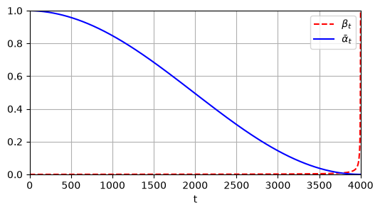
The prepare_batch() function takes a batch of images and adds noise to each of them, using a different random time between 1 and for each image, and it returns a tuple containing the inputs and the targets:
The inputs are a
dictcontaining the noisy images and the corresponding times. The function uses equation (4) from the DDPM paper to compute the noisy images in one shot, directly from the original images. It’s a shortcut for the forward diffusion process.The target is the noise that was used to produce the noisy images.
# Move the variance schedule to torch tensors, so it can be indexed with a batch of
# timesteps directly (prepare_batch and generate, below, both need this)
alpha = torch.from_numpy(alpha).to(device)
alpha_cumprod = torch.from_numpy(alpha_cumprod.astype(np.float32)).to(device)
beta = torch.from_numpy(beta).to(device)
def prepare_batch(X):
X = X.permute(0, 3, 1, 2).float() * 2 - 1 # channels-last -> channels-first, scale to [-1, +1]
batch_size = X.shape[0]
t = torch.randint(1, T + 1, (batch_size,), device=X.device)
alpha_cm = alpha_cumprod[t].view(batch_size, 1, 1, 1)
noise = torch.randn_like(X)
return {
"X_noisy": alpha_cm ** 0.5 * X + (1 - alpha_cm) ** 0.5 * noise,
"time": t,
}, noiseQ12) Prepare one DataLoader for training, and one for validation.
def prepare_dataset(X, batch_size=32, shuffle=False):
    # Create a dataset from input data
    dataset = torch.utils.data.TensorDataset(torch.from_numpy(X))

    # Return a DataLoader; shuffling and batching happen here, prepare_batch() itself
    # is called explicitly at each training step (see the training loop below)
    return torch.utils.data.DataLoader(dataset, batch_size=batch_size, shuffle=shuffle)
# Prepare the training and validation datasetsdef prepare_dataset(X, batch_size=32, shuffle=False):
# Create a dataset from input data
dataset = torch.utils.data.TensorDataset(torch.from_numpy(X))
# Return a DataLoader; shuffling and batching happen here, prepare_batch() itself
# is called explicitly at each training step (see the training loop below)
return torch.utils.data.DataLoader(dataset, batch_size=batch_size, shuffle=shuffle)
# Prepare the training and validation datasets
train_loader = prepare_dataset(X_train, batch_size=___, shuffle=___)
valid_loader = prepare_dataset(X_valid, batch_size=___)As a quick sanity check, let’s take a look at a few training samples, along with the corresponding noise to predict, and the original images (which we get by subtracting the appropriately scaled noise from the appropriately scaled noisy image):
def subtract_noise(X_noisy, time, noise):
    alpha_cm = alpha_cumprod[time].view(-1, 1, 1, 1)
    return (X_noisy - (1 - alpha_cm) ** 0.5 * noise) / alpha_cm ** 0.5

(X_batch,) = next(iter(train_loader))  # get the first batch
X_dict, Y_noise = prepare_batch(X_batch)
X_original = subtract_noise(X_dict["X_noisy"], X_dict["time"], Y_noise)
# Plot original images, noisy images and the noise to predict
def to_image_grid(X):
return ((X.permute(0, 2, 3, 1).detach().cpu().numpy() + 1) * 128).clip(0, 255).astype(np.uint8)
print("Original images")
plot_multiple_images(to_image_grid(X_original[:8]))
plt.show()
print("Time steps:", X_dict["time"].cpu().numpy()[:8])
print("Noisy images")
plot_multiple_images(to_image_grid(X_dict["X_noisy"][:8]))
plt.show()
print("Noise to predict")
plot_multiple_images(to_image_grid(Y_noise[:8]))
plt.show()Q13) Complete the diffusion model architecture below
Now we’re ready to build the diffusion model itself. It will need to process both images and times. We will encode the times using a sinusoidal encoding, as suggested in the DDPM paper, just like in the Attention is all you need paper. Given a vector of m integers representing time indices (integers), the layer returns an m × d matrix, where d is the chosen embedding size.
embed_size = 64

class TimeEncoding(nn.Module):
    def __init__(self, T, embed_size):
        super().__init__()
        assert embed_size % 2 == 0, "embed_size must be even"
        p, i = np.meshgrid(np.arange(T + 1), 2 * np.arange(embed_size // 2))
        t_emb = np.empty((T + 1, embed_size))
        t_emb[:, ::2] = np.sin(p / 10_000 ** (i / embed_size)).T
        t_emb[:, 1::2] = np.cos(p / 10_000 ** (i / embed_size)).T
        self.register_buffer("time_encodings", torch.tensor(t_emb, dtype=torch.float32))

    def forward(self, t):
        return self.time_encodings[t]
# the size of the embedding e.g. 64
embed_size = ___
# Custom module to encode time steps with sinusoidal embeddings
class TimeEncoding(nn.Module):
def __init__(self, T, embed_size):
# Initialize the module and ensure embed_size is even
super().__init__()
assert embed_size % 2 == 0, "embed_size must be even"
# Create a meshgrid for time steps and embedding indices
p, i = np.meshgrid(np.arange(T + 1), 2 * np.arange(embed_size // 2))
# Initialize the time embeddings matrix
t_emb = np.empty((T + 1, embed_size))
# Fill even indices with sine values and odd indices with cosine values
t_emb[:, ::2] = np.sin(p / 10_000 ** (i / embed_size)).T
t_emb[:, 1::2] = np.cos(p / 10_000 ** (i / embed_size)).T
# Register the embeddings as a (non-trainable) buffer
self.register_buffer("time_encodings", torch.tensor(t_emb, dtype=torch.float32))
# Method to fetch time encodings for `t` time steps
def forward(self, t):
return self.time_encodings[___]# the size of the embedding e.g. 64
embed_size = ___
# Custom module to encode time steps with sinusoidal embeddings
class TimeEncoding(nn.Module):
def __init__(self, T, embed_size):
# Initialize the module and ensure embed_size is even
super().__init__()
assert embed_size % 2 == 0, "embed_size must be even"
# Create a meshgrid for time steps and embedding indices
p, i = np.meshgrid(np.arange(T + 1), 2 * np.arange(embed_size // 2))
# Initialize the time embeddings matrix
t_emb = np.empty((T + 1, embed_size))
# Fill even indices with sine values and odd indices with cosine values
t_emb[:, ::2] = np.sin(p / 10_000 ** (i / embed_size)).T
t_emb[:, 1::2] = np.cos(p / 10_000 ** (i / embed_size)).T
# Register the embeddings as a (non-trainable) buffer
self.register_buffer("time_encodings", torch.tensor(t_emb, dtype=torch.float32))
# Method to fetch time encodings for `t` time steps
def forward(self, t):
return self.time_encodings[t]Now let’s build the model. In the Improved DDPM paper, they use a UNet model. We’ll create a UNet-like model, that processes the image through Conv2D + BatchNormalization layers and skip connections, gradually downsampling the image (using MaxPooling layers with strides=2), then growing it back again (using Upsampling2D layers). Skip connections are also added across the downsampling part and the upsampling part. We also add the time encodings to the output of each block, after passing them through a Dense layer to resize them to the right dimension.
Note: an image’s time encoding is added to every pixel in the image, along the last axis (channels). So the number of units in the
Conv2Dlayer must correspond to the embedding size, and we must reshape thetime_enctensor to add the width and height dimensions.This UNet implementation was inspired by keras.io’s image segmentation example, as well as from the official diffusion models implementation. Compared to the first implementation, I added a few things, especially time encodings and skip connections across down/up parts. Compared to the second implementation, I removed a few things, especially the attention layers. It seemed like overkill for Fashion MNIST, but feel free to add them.
class DiffusionModel(nn.Module):
    """A UNet-like model: Conv2d + BatchNorm2d blocks and skip connections, gradually
    downsampling the image (stride-2 pooling), then growing it back again (nearest-neighbor
    upsampling). Skip connections are added across the downsampling and upsampling parts.
    Time encodings are added to the output of each block, after resizing them with a Linear
    layer.

    Note: an image's time encoding is added to every pixel in the image, along the channel
    axis -- so the number of channels going into each block must match the embedding
    projection's output size.

    Unlike the reference this is adapted from (which was built for 28x28x1 Fashion MNIST),
    this version works directly on CIFAR-10's native 32x32x3 shape -- no zero-padding /
    cropping round-trip is needed since 32 is already evenly divisible by 2 three times over.
    """
    def __init__(self, T, embed_size=64, dim=16):
        super().__init__()
        self.time_encoding = TimeEncoding(T, embed_size)

        self.init_conv = nn.Conv2d(3, dim, kernel_size=3, padding=1)
        self.init_bn = nn.BatchNorm2d(dim)
        self.init_time = nn.Linear(embed_size, dim)

        down_dims = (32, 64, 128)
        in_dim = dim
        self.down_convs = nn.ModuleList()
        self.down_skips = nn.ModuleList()
        self.down_times = nn.ModuleList()
        for d in down_dims:
            self.down_convs.append(nn.ModuleList([
                nn.Conv2d(in_dim, d, kernel_size=3, padding=1),
                nn.BatchNorm2d(d),
                nn.Conv2d(d, d, kernel_size=3, padding=1),
                nn.BatchNorm2d(d),
            ]))
            self.down_skips.append(nn.Conv2d(in_dim, d, kernel_size=1, stride=2))
            self.down_times.append(nn.Linear(embed_size, d))
            in_dim = d

        up_dims = (64, 32, 16)
        cross_dims = down_dims[::-1]
        self.up_convs = nn.ModuleList()
        self.up_skiplinks = nn.ModuleList()
        self.up_times = nn.ModuleList()
        for d, cross_d in zip(up_dims, cross_dims):
            self.up_convs.append(nn.ModuleList([
                nn.ConvTranspose2d(in_dim, d, kernel_size=3, padding=1),
                nn.BatchNorm2d(d),
                nn.ConvTranspose2d(d, d, kernel_size=3, padding=1),
                nn.BatchNorm2d(d),
            ]))
            self.up_skiplinks.append(nn.Conv2d(in_dim, d, kernel_size=1))
            self.up_times.append(nn.Linear(embed_size, d))
            in_dim = d + cross_d  # after concatenating with the matching downsampling skip

        self.final_conv = nn.Conv2d(in_dim, 3, kernel_size=3, padding=1)

    def forward(self, X_noisy, time):
        # Encode the time step using the TimeEncoding module
        time_enc = self.time_encoding(time)

        # Initial convolution
        Z = F.relu(self.init_bn(self.init_conv(X_noisy)))
        # Adapt the time encoding and add it to the image feature map
        t = self.init_time(time_enc)[:, :, None, None]
        Z = Z + t

        # Keep track of skip connections and initiate a residual connection
        skip = Z
        cross_skips = []  # for skip connections in the UNet structure

        # Downsampling blocks
        for (conv1, bn1, conv2, bn2), skip_conv, time_lin in zip(
                self.down_convs, self.down_skips, self.down_times):
            Z = F.relu(bn1(conv1(Z)))
            Z = F.relu(bn2(conv2(Z)))

            # Store intermediate output for skip connection
            cross_skips.append(Z)

            # Downsample and add residual connection
            Z = F.max_pool2d(Z, kernel_size=3, stride=2, padding=1)
            skip_link = skip_conv(skip)
            Z = Z + skip_link

            # Add time information to downsampled feature maps
            t = time_lin(time_enc)[:, :, None, None]
            Z = Z + t
            skip = Z

        # Upsampling blocks
        for (convT1, bn1, convT2, bn2), skip_conv, time_lin in zip(
                self.up_convs, self.up_skiplinks, self.up_times):
            Z = F.relu(bn1(convT1(Z)))
            Z = F.relu(bn2(convT2(Z)))

            # Upsample and add residual connection
            Z = F.interpolate(Z, scale_factor=2, mode="nearest")
            skip_link = F.interpolate(skip, scale_factor=2, mode="nearest")
            skip_link = skip_conv(skip_link)
            Z = Z + skip_link

            # Add time encoding and merge with the corresponding downsampling skip connection
            t = time_lin(time_enc)[:, :, None, None]
            Z = Z + t
            Z = torch.cat([Z, cross_skips.pop()], dim=1)
            skip = Z

        # Final convolution layer
        return self.final_conv(Z)
Let’s train the model!
# Build and compile the diffusion model
model = DiffusionModel(T).to(device)
loss_fn = nn.HuberLoss()
optimizer = torch.optim.NAdam(model.parameters())

# Train the model with the training and validation datasets with e.g. 100 epochs,
# saving the best model as we go (the manual-training-loop equivalent of Keras's
# `ModelCheckpoint(save_best_only=True)`)
epochs = ___
best_val_loss = float("inf")
for epoch in range(epochs):
    model.train()
    train_losses = []
    for (X_batch,) in train_loader:
        X_dict, noise = prepare_batch(X_batch.to(device))
        optimizer.zero_grad()
        pred_noise = model(X_dict["X_noisy"], X_dict["time"])
        loss = loss_fn(pred_noise, noise)
        loss.backward()
        optimizer.step()
        train_losses.append(loss.item())

    model.eval()
    val_losses = []
    with torch.no_grad():
        for (X_batch,) in valid_loader:
            X_dict, noise = prepare_batch(X_batch.to(device))
            pred_noise = model(X_dict["X_noisy"], X_dict["time"])
            val_losses.append(loss_fn(pred_noise, noise).item())

    val_loss = np.mean(val_losses)
    print(f"Epoch {epoch + 1}/{epochs} - loss: {np.mean(train_losses):.4f} - val_loss: {val_loss:.4f}")

    if val_loss < best_val_loss:
        best_val_loss = val_loss
        torch.save(model.state_dict(), "my_diffusion_model.pth")

model.load_state_dict(torch.load("my_diffusion_model.pth"))
Now that the model is trained, we can use it to generate new images. For this, we just generate Gaussian noise, and pretend this is the result of the diffusion process, and we’re at time . Then we use the model to predict the image at time , then we call it again to get , and so on, removing a bit of noise at each step. At the end, we get an image that looks like it’s from the Fashion MNIST dataset. The equation for this reverse process is at the top of page 4 in the DDPM paper (step 4 in algorithm 2).
def generate(model, batch_size=32):
    model.eval()
    X = torch.randn(batch_size, 3, 32, 32, device=device)
    with torch.no_grad():
        for t in range(T - 1, 0, -1):
            print(f"\rt = {t}", end=" ")  # show progress
            noise = torch.randn_like(X) if t > 1 else torch.zeros_like(X)
            time_batch = torch.full((batch_size,), t, dtype=torch.long, device=device)
            X_noise = model(X, time_batch)
            X = (
                1 / alpha[t] ** 0.5
                * (X - beta[t] / (1 - alpha_cumprod[t]) ** 0.5 * X_noise)
                + (1 - alpha[t]) ** 0.5 * noise
            )
    return X
# Generate images
X_gen = generate(model)
# Plot the generated images -- move channels back to last and rescale to [0, 1] for imshow
X_gen_grid = ((X_gen.permute(0, 2, 3, 1).cpu().numpy() + 1) / 2).clip(0, 1)
plot_multiple_images(X_gen_grid, 5)
plt.show()t = 3996 t = 3992 t = 3988 t = 3984 t = 3980 t = 3976 t = 3972 t = 3968 t = 3964 t = 3960 t = 3956 t = 3952 t = 3948 t = 3944 t = 3940 t = 3936 t = 3932 t = 3928 t = 3924 t = 3920 t = 3916 t = 3912 t = 3908 t = 3904 t = 3900 t = 3896 t = 3892 t = 3888 t = 3884 t = 3880 t = 3876 t = 3872 t = 3868 t = 3864 t = 3860 t = 3856 t = 3852 t = 3848 t = 3844 t = 3840 t = 3836 t = 3832 t = 3828 t = 3824 t = 3820 t = 3816 t = 3812 t = 3808 t = 3804 t = 3800 t = 3796 t = 3792 t = 3788 t = 3784 t = 3780 t = 3776 t = 3772 t = 3768 t = 3764 t = 3760 t = 3756 t = 3752 t = 3748 t = 3744 t = 3740 t = 3736 t = 3732 t = 3728 t = 3724 t = 3720 t = 3716 t = 3712 t = 3708 t = 3704 t = 3700 t = 3696 t = 3692 t = 3688 t = 3684 t = 3680 t = 3676 t = 3672 t = 3668 t = 3664 t = 3660 t = 3656 t = 3652 t = 3648 t = 3644 t = 3640 t = 3636 t = 3632 t = 3628 t = 3624 t = 3620 t = 3616 t = 3612 t = 3608 t = 3604 t = 3600 t = 3596 t = 3592 t = 3588 t = 3584 t = 3580 t = 3576 t = 3572 t = 3568 t = 3564 t = 3560 t = 3556 t = 3552 t = 3548 t = 3544 t = 3540 t = 3536 t = 3532 t = 3528 t = 3524 t = 3520 t = 3516 t = 3512 t = 3508 t = 3504 t = 3500 t = 3496 t = 3492 t = 3488 t = 3484 t = 3480 t = 3476 t = 3472 t = 3468 t = 3464 t = 3460 t = 3456 t = 3452 t = 3448 t = 3444 t = 3440 t = 3436 t = 3432 t = 3428 t = 3424 t = 3420 t = 3416 t = 3412 t = 3408 t = 3404 t = 3400 t = 3396 t = 3392 t = 3388 t = 3384 t = 3380 t = 3376 t = 3372 t = 3368 t = 3364 t = 3360 t = 3356 t = 3352 t = 3348 t = 3344 t = 3340 t = 3336 t = 3332 t = 3328 t = 3324 t = 3320 t = 3316 t = 3312 t = 3308 t = 3304 t = 3300 t = 3296 t = 3292 t = 3288 t = 3284 t = 3280 t = 3276 t = 3272 t = 3268 t = 3264 t = 3260 t = 3256 t = 3252 t = 3248 t = 3244 t = 3240 t = 3236 t = 3232 t = 3228 t = 3224 t = 3220 t = 3216 t = 3212 t = 3208 t = 3204 t = 3200 t = 3196 t = 3192 t = 3188 t = 3184 t = 3180 t = 3176 t = 3172 t = 3168 t = 3164 t = 3160 t = 3156 t = 3152 t = 3148 t = 3144 t = 3140 t = 3136 t = 3132 t = 3128 t = 3124 t = 3120 t = 3116 t = 3112 t = 3108 t = 3104 t = 3100 t = 3096 t = 3092 t = 3088 t = 3084 t = 3080 t = 3076 t = 3072 t = 3068 t = 3064 t = 3060 t = 3056 t = 3052 t = 3048 t = 3044 t = 3040 t = 3036 t = 3032 t = 3028 t = 3024 t = 3020 t = 3016 t = 3012 t = 3008 t = 3004 t = 3000 t = 2996 t = 2992 t = 2988 t = 2984 t = 2980 t = 2976 t = 2972 t = 2968 t = 2964 t = 2960 t = 2956 t = 2952 t = 2948 t = 2944 t = 2940 t = 2936 t = 2932 t = 2928 t = 2924 t = 2920 t = 2916 t = 2912 t = 2908 t = 2904 t = 2900 t = 2896 t = 2892 t = 2888 t = 2884 t = 2880 t = 2876 t = 2872 t = 2868 t = 2864 t = 2860 t = 2856 t = 2852 t = 2848 t = 2844 t = 2840 t = 2836 t = 2832 t = 2828 t = 2824 t = 2820 t = 2816 t = 2812 t = 2808 t = 2804 t = 2800 t = 2796 t = 2792 t = 2788 t = 2784 t = 2780 t = 2776 t = 2772 t = 2768 t = 2764 t = 2760 t = 2756 t = 2752 t = 2748 t = 2744 t = 2740 t = 2736 t = 2732 t = 2728 t = 2724 t = 2720 t = 2716 t = 2712 t = 2708 t = 2704 t = 2700 t = 2696 t = 2692 t = 2688 t = 2684 t = 2680 t = 2676 t = 2672 t = 2668 t = 2664 t = 2660 t = 2656 t = 2652 t = 2648 t = 2644 t = 2640 t = 2636 t = 2632 t = 2628 t = 2624 t = 2620 t = 2616 t = 2612 t = 2608 t = 2604 t = 2600 t = 2596 t = 2592 t = 2588 t = 2584 t = 2580 t = 2576 t = 2572 t = 2568 t = 2564 t = 2560 t = 2556 t = 2552 t = 2548 t = 2544 t = 2540 t = 2536 t = 2532 t = 2528 t = 2524 t = 2520 t = 2516 t = 2512 t = 2508 t = 2504 t = 2500 t = 2496 t = 2492 t = 2488 t = 2484 t = 2480 t = 2476 t = 2472 t = 2468 t = 2464 t = 2460 t = 2456 t = 2452 t = 2448 t = 2444 t = 2440 t = 2436 t = 2432 t = 2428 t = 2424 t = 2420 t = 2416 t = 2412 t = 2408 t = 2404 t = 2400 t = 2396 t = 2392 t = 2388 t = 2384 t = 2380 t = 2376 t = 2372 t = 2368 t = 2364 t = 2360 t = 2356 t = 2352 t = 2348 t = 2344 t = 2340 t = 2336 t = 2332 t = 2328 t = 2324 t = 2320 t = 2316 t = 2312 t = 2308 t = 2304 t = 2300 t = 2296 t = 2292 t = 2289 t = 2285 t = 2281 t = 2277 t = 2273 t = 2269 t = 2265 t = 2261 t = 2257 t = 2253 t = 2249 t = 2245 t = 2241 t = 2237 t = 2233 t = 2229 t = 2225 t = 2221 t = 2217 t = 2213 t = 2209 t = 2205 t = 2201 t = 2197 t = 2193 t = 2189 t = 2185 t = 2181 t = 2177 t = 2173 t = 2169 t = 2165 t = 2161 t = 2157 t = 2153 t = 2149 t = 2145 t = 2141 t = 2137 t = 2133 t = 2129 t = 2125 t = 2121 t = 2117 t = 2113 t = 2109 t = 2105 t = 2101 t = 2097 t = 2093 t = 2089 t = 2085 t = 2081 t = 2077 t = 2073 t = 2069 t = 2065 t = 2061 t = 2057 t = 2053 t = 2049 t = 2045 t = 2041 t = 2037 t = 2033 t = 2029 t = 2025 t = 2021 t = 2017 t = 2013 t = 2009 t = 2005 t = 2001 t = 1997 t = 1993 t = 1989 t = 1985 t = 1981 t = 1977 t = 1973 t = 1969 t = 1965 t = 1961 t = 1957 t = 1953 t = 1949 t = 1945 t = 1941 t = 1937 t = 1933 t = 1929 t = 1925 t = 1921 t = 1917 t = 1913 t = 1909 t = 1905 t = 1901 t = 1897 t = 1893 t = 1889 t = 1885 t = 1881 t = 1877 t = 1873 t = 1869 t = 1866 t = 1862 t = 1858 t = 1854 t = 1850 t = 1846 t = 1842 t = 1838 t = 1834 t = 1830 t = 1826 t = 1822 t = 1818 t = 1814 t = 1810 t = 1806 t = 1802 t = 1798 t = 1794 t = 1790 t = 1786 t = 1782 t = 1778 t = 1774 t = 1770 t = 1766 t = 1762 t = 1758 t = 1754 t = 1750 t = 1746 t = 1742 t = 1738 t = 1734 t = 1730 t = 1726 t = 1722 t = 1718 t = 1714 t = 1710 t = 1706 t = 1702 t = 1698 t = 1694 t = 1690 t = 1686 t = 1682 t = 1678 t = 1674 t = 1670 t = 1666 t = 1662 t = 1658 t = 1654 t = 1650 t = 1646 t = 1642 t = 1638 t = 1634 t = 1630 t = 1626 t = 1622 t = 1618 t = 1614 t = 1610 t = 1606 t = 1602 t = 1598 t = 1594 t = 1590 t = 1586 t = 1582 t = 1578 t = 1574 t = 1570 t = 1566 t = 1562 t = 1558 t = 1554 t = 1550 t = 1546 t = 1542 t = 1538 t = 1534 t = 1530 t = 1526 t = 1522 t = 1518 t = 1514 t = 1510 t = 1506 t = 1502 t = 1498 t = 1494 t = 1490 t = 1486 t = 1482 t = 1478 t = 1474 t = 1470 t = 1466 t = 1462 t = 1458 t = 1454 t = 1450 t = 1446 t = 1442 t = 1438 t = 1434 t = 1430 t = 1426 t = 1422 t = 1418 t = 1414 t = 1410 t = 1406 t = 1402 t = 1398 t = 1394 t = 1390 t = 1386 t = 1382 t = 1378 t = 1374 t = 1370 t = 1366 t = 1362 t = 1358 t = 1354 t = 1350 t = 1346 t = 1342 t = 1338 t = 1334 t = 1330 t = 1326 t = 1322 t = 1318 t = 1314 t = 1310 t = 1306 t = 1302 t = 1298 t = 1294 t = 1290 t = 1286 t = 1282 t = 1278 t = 1274 t = 1270 t = 1266 t = 1262 t = 1258 t = 1254 t = 1250 t = 1246 t = 1242 t = 1238 t = 1234 t = 1230 t = 1226 t = 1222 t = 1218 t = 1214 t = 1210 t = 1206 t = 1202 t = 1198 t = 1194 t = 1190 t = 1186 t = 1182 t = 1178 t = 1174 t = 1170 t = 1166 t = 1162 t = 1158 t = 1154 t = 1150 t = 1146 t = 1142 t = 1138 t = 1134 t = 1130 t = 1126 t = 1122 t = 1118 t = 1114 t = 1110 t = 1106 t = 1102 t = 1098 t = 1094 t = 1090 t = 1086 t = 1082 t = 1078 t = 1074 t = 1070 t = 1066 t = 1062 t = 1058 t = 1054 t = 1050 t = 1046 t = 1042 t = 1038 t = 1034 t = 1030 t = 1026 t = 1022 t = 1018 t = 1014 t = 1010 t = 1006 t = 1002 t = 998 t = 994 t = 990 t = 986 t = 982 t = 978 t = 974 t = 970 t = 966 t = 962 t = 958 t = 954 t = 950 t = 946 t = 942 t = 938 t = 934 t = 930 t = 926 t = 922 t = 918 t = 914 t = 910 t = 906 t = 902 t = 898 t = 894 t = 890 t = 886 t = 882 t = 878 t = 874 t = 870 t = 866 t = 862 t = 858 t = 854 t = 850 t = 846 t = 842 t = 838 t = 834 t = 830 t = 826 t = 822 t = 818 t = 814 t = 810 t = 806 t = 802 t = 798 t = 794 t = 790 t = 786 t = 782 t = 778 t = 774 t = 770 t = 766 t = 762 t = 758 t = 754 t = 750 t = 746 t = 742 t = 738 t = 734 t = 730 t = 726 t = 722 t = 718 t = 714 t = 710 t = 706 t = 702 t = 698 t = 694 t = 690 t = 686 t = 682 t = 678 t = 674 t = 670 t = 666 t = 662 t = 658 t = 654 t = 650 t = 646 t = 642 t = 638 t = 634 t = 630 t = 626 t = 622 t = 618 t = 614 t = 610 t = 606 t = 602 t = 598 t = 594 t = 590 t = 586 t = 582 t = 578 t = 574 t = 570 t = 566 t = 562 t = 558 t = 554 t = 550 t = 546 t = 542 t = 538 t = 534 t = 530 t = 526 t = 522 t = 518 t = 514 t = 510 t = 506 t = 502 t = 498 t = 494 t = 490 t = 486 t = 482 t = 478 t = 474 t = 470 t = 466 t = 462 t = 458 t = 454 t = 450 t = 446 t = 442 t = 438 t = 434 t = 430 t = 426 t = 422 t = 418 t = 414 t = 410 t = 406 t = 402 t = 398 t = 394 t = 390 t = 386 t = 382 t = 378 t = 374 t = 370 t = 366 t = 362 t = 358 t = 354 t = 350 t = 346 t = 342 t = 338 t = 334 t = 330 t = 326 t = 322 t = 318 t = 314 t = 310 t = 306 t = 302 t = 298 t = 294 t = 290 t = 286 t = 282 t = 278 t = 274 t = 270 t = 266 t = 262 t = 258 t = 254 t = 250 t = 246 t = 242 t = 238 t = 234 t = 230 t = 226 t = 222 t = 218 t = 214 t = 210 t = 206 t = 202 t = 198 t = 194 t = 190 t = 186 t = 182 t = 178 t = 174 t = 170 t = 166 t = 162 t = 158 t = 154 t = 150 t = 146 t = 142 t = 138 t = 134 t = 130 t = 126 t = 122 t = 118 t = 114 t = 110 t = 106 t = 102 t = 98 t = 94 t = 90 t = 86 t = 82 t = 78 t = 74 t = 70 t = 66 t = 62 t = 58 t = 54 t = 50 t = 46 t = 42 t = 38 t = 34 t = 30 t = 26 t = 22 t = 18 t = 14 t = 10 t = 6 t = 2 t = 1 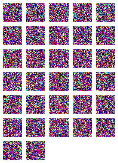
Some of these images are really convincing! Compared to GANs, diffusion models tend to generate more diverse images, and they have surpassed GANs in image quality. Moreover, training is much more stable. However, generating images takes much longer.
Faster sampling with DDIM
generate() calls the model once per timestep: 4000 forward passes for a single batch of
images, which is why sampling takes so much longer than it does with a GAN. Denoising
diffusion implicit models (DDIM) keep the network exactly as it is and shorten the path
instead. Pick a subsequence of the training timesteps — say 50 of the 4000 — and at each one,
rearrange the forward-process equation to recover the model’s implied estimate of the clean
image, then re-noise that estimate straight to the next timestep in the subsequence, skipping
everything in between.
The forward process defines the noisy image at time as
so given and the noise the model predicts, the implied clean image is — and re-noising it to any earlier timestep is the same equation run forwards again with .
No retraining is involved: this uses the weights trained above. Two things change. Sampling is 80 times cheaper at 50 steps, and it is deterministic — no fresh Gaussian noise is drawn inside the loop, so the same starting noise always gives the same image.
Q14) Generate images from the trained model in 50 steps instead of 4000
def generate_ddim(model, batch_size=32, n_steps=50):
    """Sample with DDIM: the trained model, evaluated on a subsequence of timesteps."""
    model.eval()
    X = torch.randn(batch_size, 3, 32, 32, device=device)

    # a decreasing subsequence of the T training timesteps, e.g. 4000, 3918, ..., 1
    times = torch.linspace(T, 1, n_steps).long().tolist()

    with torch.no_grad():
        # pair each timestep with the one it jumps to; the last jump lands on 0, and
        # alpha_cumprod[0] is 1, which is the clean image
        for t, t_prev in zip(times, times[1:] + [0]):
            time_batch = torch.full((batch_size,), t, dtype=torch.long, device=device)
            X_noise = model(X, time_batch)

            # invert the forward process to get the clean image the model implies,
            # then re-noise it to t_prev rather than stepping through every timestep
            X_start = (X - (1 - alpha_cumprod[t]) ** 0.5 * X_noise) / alpha_cumprod[t] ** 0.5
            X_start = X_start.clamp(-1, 1)          # the estimate can drift outside the data range
            X = alpha_cumprod[t_prev] ** 0.5 * X_start + (1 - alpha_cumprod[t_prev]) ** 0.5 * X_noise

    return X
# Generate with the same trained model, timing both samplers to see the difference
import time

start = time.time()
X_gen_ddim = generate_ddim(model, n_steps=___)
print(f"DDIM: {time.time() - start:.1f} s")

X_gen_ddim_grid = ((X_gen_ddim.permute(0, 2, 3, 1).cpu().numpy() + 1) / 2).clip(0, 1)
plot_multiple_images(X_gen_ddim_grid, 5)
plt.show()
With 50 steps the images are a little smoother and lose some fine detail compared with the full
4000-step run, and they arrive in seconds rather than minutes. Raising n_steps trades that
speed back for detail, so it is worth generating the same batch at 20, 50 and 200 steps and
comparing — the starting noise is the only randomness, so fixing the seed makes the three
directly comparable.