3.2) (Exercises) Support Vector Machines

Now that you have learned the basics of Support Vector Machines and tuning regularization parameters can make the trained SVMs more generalizable, it is time to learn how to create and train a simple SVM.

We will start with a sample dataset including measurements of different physical characteristics of flowers. We would like to train a support vector machine to automatically differentiate two different types of flowers. After training our first SVM model, we will make additional experiments to see how the decision boundaries of regularized versions of trained SVMs differ from less regularized ones.

Goal: Building similar models based on different types of Support Vector Machines (SVMs) to classify linearly separable classes, here Iris Setosa and Iris Versicolor from the Iris dataset.

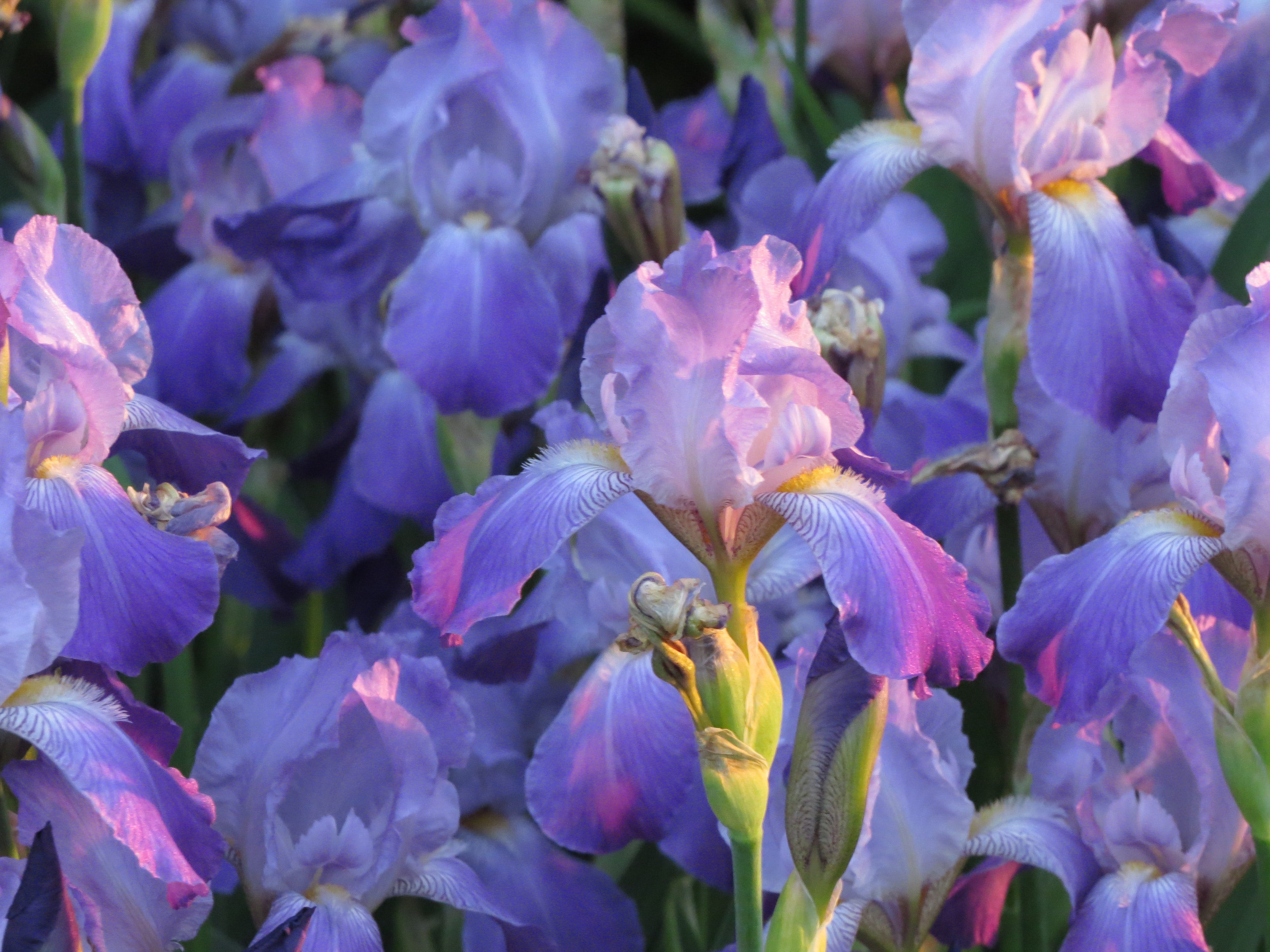
Caption: Iris flowers in the evening light. Are they Irises Setosa or Irises Versicolor?

Source: Photo by Christina Brinza on Unsplash

First, let’s load the Iris dataset! 💐

from sklearn import datasets # Import datasets from scikit-learn
import matplotlib.pyplot as plt
import numpy as np

iris = datasets.load_iris() # Load the Iris dataset specifically
X = iris["data"][:, (2, 3)]  # Features = petal length, petal width
y = iris["target"] # Target = Iris species

# The iris dataset contains information of different types of flowers.
# Here we want to choose two flowers: setosa and versicolor

setosa_or_versicolor = (y == 0) | (y == 1) # Indices of Irises setosa/versicolor
X = X[setosa_or_versicolor] # Only keep Irises setosa/versicolor in features
y = y[setosa_or_versicolor] # Only keep Irises setosa/versicolor in target

Now we have our pre-processed dataset 💐:

Our features are (petal length, petal width) in X.

Our target is (Iris species) in y.

# (Optional) Expore X and y to familiarize yourself
# with the pre-processed dataset
# A couple of things you can try is to look the size of the dataset you just loaded.
# (e.g., X.shape, y.shape)

Q1) Train a Linear Support Vector Classification model on the pre-processed dataset

Hint: The documentation for LinearSVC is at this link

# Import the LinearSVC class from the scikit-learn `svm` library
from sklearn.___ import ___________

# Fit a LinearSVC object on the Iris dataset
# (1) Initiate a LinearSVC object
______ = ________
# (2) Use the LinearSVC object to fit the dataset you just created. Use .fit() for this task.
______.___(__,__)

Q2) Plot the decision boundary of this classifier

Hint: According to the documentation, given a SVC object svc:

Weights: W = svc.coef_[0], and
Intercept: I = svc.intercept_

the decision boundary is the line:

$y_{boundary} = -\frac{W\left[0\right] x + I\left[0\right]}{W\left[1\right]}$

⚠ If you normalized your inputs before feeding it to the SVM in the previous question (e.g., via the StandardScaler), the equation above is only valid in “normalized” coordinates.

# Use the first part of the hint to get the weights of the fitted SVC object
W = ____._____
# Use the second part of the hint to get the intercept of the fitted SVC object
I = ____._____

Now show the decision boundary that you just got in a scatter plot. Can it cleanly separate different flowers?

Hint: (1) We will use plt.scatter() to plot the flower data. Check documentation for details. (2) We will need to initiate a X array to plot the decision boundary. There are many ways to create such an array, but let’s use np.linspace() for now. Documentation

# On the same figure: Scatter the features X and plot the decision boundary
# Don't forget to label the axes and add a legend to your figure
# Initiate a figure using plt.subplots
___,ax = plt.subplots(__,___)

# Now plot all feature Xs in a scatter plot. Use these settings:
# (s = 80, color='r', edgecolor='k', linewidths=1.5)
# X, y indices of the inputs can be accessed like this X[:,0] [X indices]; X[:,1] [Y indices]
ax.________(______,________,s=___,color=___,edgecolor=___,linewidths=___)

# Decision boundary: yboundary = - (W[0]*x+I[0])/W[1]
# Initiate a 1D array X with np.linspace()
x = np.linspace(_____)
# Calculate yboundary
yboundary = ___________
plt.plot(___,____,c='r',lw=2)

ax.set_xlabel("Pedal length",fontdict={'size':13})
ax.set_ylabel("Pedal width",fontdict={'size':13})
ax.set_title('Iris dataset')
ax.tick_params(axis='both', which='major', labelsize=11)
ax.grid(alpha=0.2,ls='--',lw=1)
#[x.set_linewidth(2) for x in ax.spines.values()]
plt.show()

Q3) Train a SVC and a SGDClassifier for the same task and compare these two models to the LinearSVC. Use kernel = 'Linear' when instantiating the SVC!

Hint: Here is the documentation for the SVC class and the SGDClassifier class.

# Import SVC and SGDClassifier
from sklearn.___ import _____ #SVC
from sklearn.__________ import ______________ #SGDClassifier

# Fit the `SVC` and the `SGDClassifier` to the pre-processed dataset
# Instantiate 'SVC', use kernel='linear'
______ = SVC(_____________)
# Instantiate 'SGDClassifier'
______ = __________()

# Fit models with data
______.____(_,_) # SVC
______.____(_,_)

# Plot all three decision boundaries on the same labeled figure
#########################################################################
# Same as what you did to get the first figure
___,___ = ______.____________(____,____)
ax.scatter(________________________)

# Decision boundary: np.dot(W,x)+b = 0
_ = ________(_______)
__._____(_,_________,c='r',lw=2,label='LinearSVC')
#########################################################################
# Now add the decision boundary for 'SVC'
__._____(_,______________________,c='k',lw=2,label='SVC')
#########################################################################
# Now add the decision boundary for 'SGDClassifier'
__._____(_,______________________,c='b',lw=2,label='SGDClas.')
#########################################################################
# Same as the first figure again
ax.legend()
ax.set_xlabel("Pedal length",fontdict={'size':13})
ax.set_ylabel("Pedal width",fontdict={'size':13})
ax.set_title('Iris dataset')
ax.tick_params(axis='both', which='major', labelsize=11)
ax.grid(alpha=0.2,ls='--',lw=1)
plt.show()

Q4) Create more regularized versions of each model and compare these new models to the previous ones

Hint: Vary the hyperparameter C for the LinearSVC and SVC models, and vary the hyperparameter alpha for the SGDClassifier model. Consult the documentation to know whether to increase or decrease the regularization parameters.

# Fit more regularized versions of the `LinearSVC` model
irisSVC_r = LinearSVC(C=_____).fit(X,y)

# Fit more regularized versions of the `SVC` model
irisSVC2_r = SVC(C=_____,______='_____').fit(X,y)

# Fit more regularized versions of the `SGDClassifier` model
irisSGDc_r = SGDClassifier(alpha=_________).fit(X,y)

# Compare the new decision boundaries to the old ones
# Plot all three decision boundaries on the same labeled figure
#########################################################################
# Same as what you did to get the second figure
___,___ = ______.____________(____,____)
ax.scatter(________________________)

# Decision boundary: np.dot(W,x)+b = 0
_ = ________(_______)
__._____(_,_________,c='r',lw=2,label='LinearSVC')
__._____(_,______________________,c='k',lw=2,label='SVC')
__._____(_,______________________,c='b',lw=2,label='SGDClas.')
#########################################################################
# Now add the decision boundaries for the regularized models
# Regularized LinearSVC model
# Find the weights and intercept
Wlsvc_r,Ilsvc_r = _____________,_____________
ax.plot(x,_____________________________,c='r',lw=2,ls='--',label='LinearSVC_r')
# Regularized SVC model
# Find the weights and intercept
Wsvc_r,Isvc_r = _____________,_____________
ax.plot(x,_____________________________,c='k',lw=2,ls='--',label='SVC_r')
# Regularized SGDClassifier model
# Find the weights and intercept
Wsgdc_r,Isgdc_r = _____________,_____________
ax.plot(x,_____________________________,c='b',lw=2,ls='--',label='SGDClas._r')
#########################################################################
# Same as what you did to get the second figure
ax.legend()
ax.set_xlabel("Pedal length",fontdict={'size':13})
ax.set_ylabel("Pedal width",fontdict={'size':13})
ax.set_title('Iris dataset')
ax.tick_params(axis='both', which='major', labelsize=11)
ax.grid(alpha=0.2,ls='--',lw=1)
plt.show()

How does regularization affect the decision boundary in this simple case?

Bonus Exercise 1: Training a SVM Regressor on the California Housing Dataset¶

Can we use SVMs to predict the price of a house in California (in 1990) based on its characteristics (longitude, latitude, total_rooms, etc.)?

The dataset was originally used in Pace, R. Kelley, and Ronald Barry. “Sparse spatial autoregressions.” Statistics & Probability Letters 33.3 (1997): 291-297.

Let’s first load the dataset using Scikit-Learn’s fetch_california_housing() function:

from sklearn.datasets import fetch_california_housing # Import function

housing = fetch_california_housing() # Fetch dataset
X = housing["data"] # Features
y = housing["target"] # Targets

# Don't hesitate to do some preliminary data analysis here

Let’s split the data into a training set and a test set:

from sklearn.model_selection import train_test_split # Import function
# from scikit-learn

# Split the dataset into training and test sets
X_train, X_test, y_train, y_test = train_test_split(X, y,
                                                    test_size=0.2,
                                                    random_state=42)

Q1) Normalize the features X before training the regressor

Hint: You may use the StandardScaler to normalize X using its z-score.

# Define the normalization/scaler

# Normalize the features `X`

Q2) Start by training a simple Linear Support Vector Regression and assess its performance on the training and test sets

Hint 1: Here’s the documentation for scikit-learn’s LinearSVR

Hint 2: You may assess the regressor’s performance using the any scikit-learn regression metric you find interpretable.

# Train a simple linear SVR

# Assess its performance on the training and test sets

Q3) How large is the model error in $?

Hint: The unit of y in the dataset is $10,000.

# Estimate the approximate model error in units 10,000$

Q4) Try to beat your linear model using more complex SVM regressors.

Hint 1: The performance of a model should be assessed using the test set.

Hint 2: Géron’s model uses a SVR for which the hyperparameters gamma and C were optimized using a Randomized Search, and gets the root mean-squared error down to approximately 6,000 dollars on the test dataset.

# Experiment here

# Have fun

# But don't spend too too much time on it as we have two more exercises
# to go through before we get to the wildfire dataset