


Figure: An AI artwork on GNN and weather forcasting created by GPT4, 2024
This notebook is designed to be run on Google Colab and we highly recommend clicking on the Google Colab badge above.
To start, we will load a classic graph in network science, the Karate Club Network. Then we will offer the basic tutorial for NetworkX before exploring multiple graph statistics.
With the help of the PyTorch Geometric tutorial, we will then work together to transform the graph structure into a PyTorch tensor, enabling machine learning applications.
And we will finish the first learning algorithm on graphs: a node embedding model. For simplicity, our model here is simpler than classical algorithms applied in the research, such as DeepWalk or node2vec. But it’s still rewarding and challenging, as we will write it from scratch via PyTorch.
Finally, we will implement one of the simplest GNN operators, the Graph Convolutional Networks (Kipf et al. (2017)). We hope you can use this 3-layers GCN to learn embeddings that will be useful to classify each node into its community within the Karate Club Network.
8.2.1 Graph Basics
To start, we will load a classic graph in network science, the Karate Club Network. We will explore multiple graph statistics for that graph.
NetworkX Tutorial
NetworkX is one of the most frequently used Python packages to create, manipulate, and mine graphs.
This tutorial is adapted from jdwittenauer’s NetworkX notebook.
You can explore more NetworkX functions through its documentation.
Setup
# Install/upgrade packages
!pip install --upgrade scipy networkx
Defaulting to user installation because normal site-packages is not writeable
Collecting scipy
  Downloading scipy-1.18.1-cp312-cp312-manylinux_2_27_x86_64.manylinux_2_28_x86_64.whl.metadata (62 kB)
     ━━━━━━━━━━━━━━━━━━━━━━━━━━━━━━━━━━━━━━━━ 0.0/62.4 kB ? eta -:--:--
━━━━━━━━━━━━━━━━━━━━━━━━━━━━━━━━━━━━━━━━ 62.4/62.4 kB 4.8 MB/s eta 0:00:00
Collecting networkx
Downloading networkx-3.7-py3-none-any.whl.metadata (6.7 kB)
Collecting numpy<2.8,>=2.0.0 (from scipy)
  Downloading numpy-2.5.3-cp312-cp312-manylinux_2_27_x86_64.manylinux_2_28_x86_64.whl.metadata (6.6 kB)
Downloading scipy-1.18.1-cp312-cp312-manylinux_2_27_x86_64.manylinux_2_28_x86_64.whl (35.3 MB)
━━━━━━━━━━━━━━━━━━━━━━━━━━━━━━━━━━━━━━━━ 0.0/35.3 MB ? eta -:--:-- ━━━━━━━╸━━━━━━━━━━━━━━━━━━━━━━━━━━━━━━━━ 6.7/35.3 MB 203.9 MB/s eta 0:00:01 ━━━━━━━━━━━━━━━━━━━━━╺━━━━━━━━━━━━━━━━━━ 18.9/35.3 MB 169.6 MB/s eta 0:00:01 ━━━━━━━━━━━━━━━━━━━━━━━━━━━━━━╺━━━━━━━━━ 26.9/35.3 MB 236.0 MB/s eta 0:00:01 ━━━━━━━━━━━━━━━━━━━━━━━━━━━━━━━━━━━━━━━╸ 35.3/35.3 MB 249.8 MB/s eta 0:00:01 ━━━━━━━━━━━━━━━━━━━━━━━━━━━━━━━━━━━━━━━━ 35.3/35.3 MB 120.8 MB/s eta 0:00:0000:01
Downloading networkx-3.7-py3-none-any.whl (2.1 MB)
━━━━━━━━━━━━━━━━━━━━━━━━━━━━━━━━━━━━━━━━ 2.1/2.1 MB 161.5 MB/s eta 0:00:00
Downloading numpy-2.5.3-cp312-cp312-manylinux_2_27_x86_64.manylinux_2_28_x86_64.whl (16.7 MB)
━━━━━━━━━━━━━━━━━━━━━━━━━━━━━━━━━━━━━━━━ 0.0/16.7 MB ? eta -:--:-- ━━━━━━━━━━━━━━━━━━╸━━━━━━━━━━━━━━━━━━━━━ 7.9/16.7 MB 236.3 MB/s eta 0:00:01 ━━━━━━━━━━━━━━━━━━━━━━━━━━━━━━━━━━━━━━━━ 16.7/16.7 MB 152.3 MB/s eta 0:00:00a 0:00:01
Installing collected packages: numpy, networkx, scipy
Successfully installed networkx-3.7 numpy-2.5.3 scipy-1.18.1
# Import the NetworkX package
import networkx as nxGraph
NetworkX provides several classes to store different types of graphs, such as directed and undirected graphs. It also provides classes to create multigraphs (both directed and undirected).
For more information, please refer to NetworkX graph types.
# Create an undirected graph G
G = nx.Graph()
print(G.is_directed())

# Create a directed graph H
H = nx.DiGraph()
print(H.is_directed())

# Add graph level attribute
G.graph["Name"] = "Bar"
print(G.graph)
False
True
{'Name': 'Bar'}
Node
Nodes (with attributes) can be easily added to NetworkX graphs.
# Add one node with node level attributes
G.add_node(0, feature=5, label=0)

# Get attributes of the node 0
node_0_attr = G.nodes[0]
print("Node 0 has the attributes {}".format(node_0_attr))
Node 0 has the attributes {'feature': 5, 'label': 0}
G.nodes(data=True)NodeDataView({0: {'feature': 5, 'label': 0}})# Add multiple nodes with attributes
G.add_nodes_from([
(1, {"feature": 1, "label": 1}),
(2, {"feature": 2, "label": 2})
]) #(node, attrdict)
# Loop through all the nodes
# Set data=True will return node attributes
for node in G.nodes(data=True):
print(node)
# Get number of nodes
num_nodes = G.number_of_nodes()
print("G has {} nodes".format(num_nodes))(0, {'feature': 5, 'label': 0})
(1, {'feature': 1, 'label': 1})
(2, {'feature': 2, 'label': 2})
G has 3 nodes
Edge
Similar to nodes, edges (with attributes) can also be easily added to NetworkX graphs.
# Add one edge with edge weight 0.5
G.add_edge(0, 1, weight=0.5)

# Get attributes of the edge (0, 1)
edge_0_1_attr = G.edges[(0, 1)]
print("Edge (0, 1) has the attributes {}".format(edge_0_1_attr))
Edge (0, 1) has the attributes {'weight': 0.5}
# Add multiple edges with edge weights
G.add_edges_from([
  (1, 2, {"weight": 0.3}),
  (2, 0, {"weight": 0.1})
])

# Loop through all the edges
# Here there is no data=True, so only the edge will be returned
for edge in G.edges():
  print(edge)

# Get number of edges
num_edges = G.number_of_edges()
print("G has {} edges".format(num_edges))
(0, 1)
(0, 2)
(1, 2)
G has 3 edges
Graph Visualization
NetworkX also provides tooling to conventiently visualize graphs.
# Draw the graph
nx.draw(G, with_labels = True)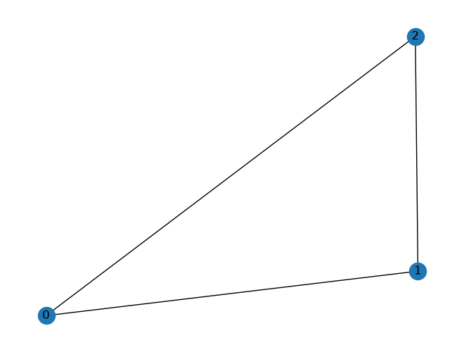
Node Degree and Neighbor
node_id = 1

# Degree of node 1
print("Node {} has degree {}".format(node_id, G.degree[node_id]))

# Get neighbor of node 1
for neighbor in G.neighbors(node_id):
  print("Node {} has neighbor {}".format(node_id, neighbor))
Node 1 has degree 2
Node 1 has neighbor 0
Node 1 has neighbor 2
Other Functionalities
NetworkX also provides plenty of useful methods to study graphs. Here is an example of getting the PageRank value of nodes (we will implement PageRank ourselves later in this notebook).
num_nodes = 4

# Create a new path like graph and change it to a directed graph
G = nx.DiGraph(nx.path_graph(num_nodes))
nx.draw(G, with_labels = True)

# Get the PageRank
pr = nx.pagerank(G, alpha=0.8)
pr
{0: 0.17857162031103999,
1: 0.32142837968896,
2: 0.32142837968896,
3: 0.17857162031103999}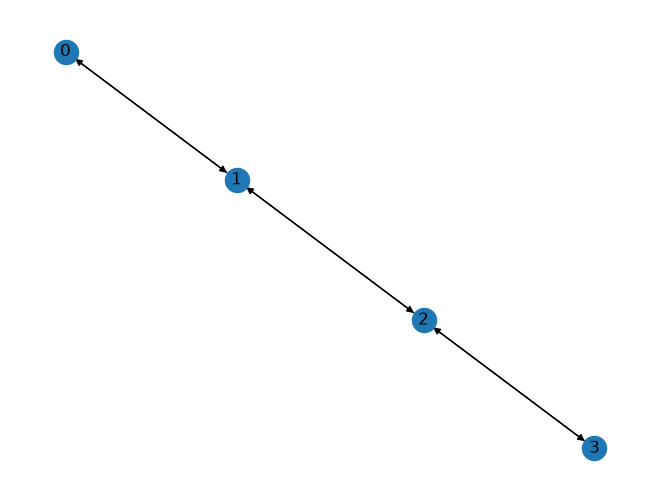
Exercise 1
Zachary’s karate club network
The Karate Club Network is a graph which describes a social network of 34 members of a karate club and documents links between members who interacted outside the club.
# Find the karate club network from the NetworkX
G_karate = nx.karate_club_graph()

# G is an undirected graph
type(G_karate)

# Visualize the graph
nx.draw(G_karate, with_labels = True)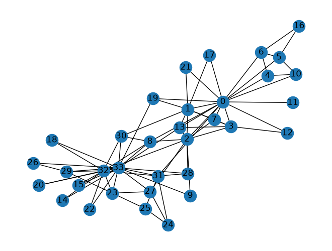
Question 1: What is the average degree of the karate club network?
def average_degree(num_edges, num_nodes):
  # TODO: Implement this function that takes number of edges
  # and number of nodes, and returns the average node degree of
  # the graph. Round the result to nearest integer (for example
  # 3.3 will be rounded to 3 and 3.7 will be rounded to 4)

  avg_degree = 0

  ############# Your code here ############
  #########################################

  return avg_degree
num_edges = G_karate.number_of_edges()
num_nodes = G_karate.number_of_nodes()
avg_degree = average_degree(num_edges, num_nodes)
print("Average degree of karate club network is {}".format(avg_degree))Average degree of karate club network is 0
Question 2: What is the average clustering coefficient of the karate club network?
def average_clustering_coefficient(G_karate):
  # TODO: Implement this function that takes a nx.Graph
  # and returns the average clustering coefficient. Round
  # the result to 2 decimal places (for example 3.333 will
  # be rounded to 3.33 and 3.7571 will be rounded to 3.76)

  avg_cluster_coef = 0

  ############# Your code here ############
  ## Note:
  ## 1: Please use the appropriate NetworkX clustering function
  #########################################

  return avg_cluster_coef
avg_cluster_coef = average_clustering_coefficient(G_karate)
print("Average clustering coefficient of karate club network is {}".format(avg_cluster_coef))Average clustering coefficient of karate club network is 0
Question 3: What is the PageRank value for node 0 (node with id 0) after one PageRank iteration?
Page Rank measures importance of nodes in a graph using the link structure of the web. A “vote” from an important page is worth more. Specifically, if a page with importance has out-links, then each link gets votes. Thus, the importance of a Page , represented as is the sum of the votes on its in links.
where is the out degree of node .
The PageRank algorithm (used by Google) outputs a probability distribution which represent the likelihood of a random surfer clicking on links will arrive at any particular page. At each time step, the random surfer has two options
With prob. , follow a link at random
With prob. , jump to a random page
Thus, the importance of a particular page is calculated with the following PageRank equation:
Please complete the code block by implementing the above PageRank equation for node 0.
Note: You can refer to more information from Stanford CS224W’s PageRank slides
def one_iter_pagerank(G_karate, beta, r0, node_id):
  # TODO: Implement this function that takes a nx.Graph, beta, r0 and node id.
  # The return value r1 is the one interation PageRank value for the input node.
  # Please round r1 to 2 decimal places.

  r1 = 0

  ############# Your code here ############
  ## Note:
  ## 1: You should not use nx.pagerank
  #########################################

  return r1
beta = 0.8
r0 = 1 / G_karate.number_of_nodes()
node = 0
r1 = one_iter_pagerank(G_karate, beta, r0, node)
print("The PageRank value for node 0 after one iteration is {}".format(r1))The PageRank value for node 0 after one iteration is 0
Question 4: What is the (raw) closeness centrality for the karate club network node 5?
The equation for closeness centrality is
def closeness_centrality(G_karate, node=5):
  # TODO: Implement the function that calculates closeness centrality
  # for a node in karate club network. G is the input karate club
  # network and node is the node id in the graph. Please round the
  # closeness centrality result to 2 decimal places.

  closeness = 0

  ## Note:
  ## 1: You can use networkx closeness centrality function.
  ## 2: Notice that networkx closeness centrality returns the normalized
  ## closeness directly, which is different from the raw (unnormalized)
  ## one that we learned in the lecture.
  #########################################

  return closeness
node = 5
closeness = closeness_centrality(G_karate, node=node)
print("The node 5 has closeness centrality {}".format(closeness))The node 5 has closeness centrality 0
8.2.2 Graph to Tensor
We will then work together to transform the graph into a PyTorch tensor, so that we can perform machine learning over the graph.
PyTorch Geometric Tutorial
PyTorch Geometric (PyG) is an extension library for PyTorch. It provides useful primitives to develop Graph Deep Learning models, including various graph neural network layers and a large number of benchmark datasets.
Don’t worry if you don’t understand some concepts such as GCNConv, as it may not be immediately useful depending on your exact objectives.
This tutorial is adapted from PyG’s own “Introduction: Hands-on Graph Neural Networks” Colab by Matthias Fey.
You can explore more PyG functions through its documentation.
import torch

print("PyTorch has version {}".format(torch.__version__))
PyTorch has version 2.14.0+cu130
Installing dependencies
Execute the cell below to install PyTorch Geometric -- in case of issues, more information can be found on PyG’s installation page. Since PyG 2.3, the base package works standalone with just PyTorch, so no separate torch-scatter/torch-sparse wheels are needed for this notebook.
# Install torch geometric
!pip install -q torch_geometric
PyTorch tensor basics
Recently, deep learning on graphs has emerged to one of the hottest research fields in the deep learning community. Here, Graph Neural Networks (GNNs) aim to generalize classical deep learning concepts to irregular structured data (in contrast to images or texts) and to enable neural networks to reason about objects and their relations.
This tutorial will introduce you to some fundamental concepts regarding deep learning on graphs via Graph Neural Networks based on the PyTorch Geometric (PyG) library. PyTorch Geometric is an extension library to the popular deep learning framework PyTorch, and consists of various methods and utilities to ease the implementation of Graph Neural Networks.
We can generate PyTorch tensor with all zeros, ones or random values.
# Generate 3 x 4 tensor with all ones
ones = torch.ones(3, 4)
print(ones)

# Generate 3 x 4 tensor with all zeros
zeros = torch.zeros(3, 4)
print(zeros)

# Generate 3 x 4 tensor with random values on the interval [0, 1)
random_tensor = torch.rand(3, 4)
print(random_tensor)

# Get the shape of the tensor
print(ones.shape)
tensor([[1., 1., 1., 1.],
[1., 1., 1., 1.],
[1., 1., 1., 1.]])
tensor([[0., 0., 0., 0.],
[0., 0., 0., 0.],
[0., 0., 0., 0.]])
tensor([[0.1184, 0.2349, 0.1193, 0.4605],
[0.3441, 0.8413, 0.3622, 0.9266],
[0.6594, 0.3176, 0.3243, 0.0545]])
torch.Size([3, 4])
PyTorch tensor contains elements for a single data type, the dtype.
# Create a 3 x 4 tensor with all 32-bit floating point zeros
zeros = torch.zeros(3, 4, dtype=torch.float32)
print(zeros.dtype)

# Change the tensor dtype to 64-bit integer
zeros = zeros.type(torch.long)
print(zeros.dtype)
torch.float32
torch.int64
Dataset
Following Kipf et al. (2017), let’s dive into the world of GNNs by looking at a simple graph-structured and previous example that we used, the well-known Zachary’s karate club network. Here, we are interested in detecting communities that arise from the member’s interaction.
PyTorch Geometric provides an easy access to the dataset via the torch_geometric.datasets subpackage:
from torch_geometric.datasets import KarateClub

dataset = KarateClub()
print(f'Dataset: {dataset}:')
print('======================')
print(f'Number of graphs: {len(dataset)}')
print(f'Number of features: {dataset.num_features}')
print(f'Number of classes: {dataset.num_classes}')
After initializing the KarateClub dataset, we first can inspect some of its properties.
For example, we can see that this dataset holds exactly one graph, and that each node in this dataset is assigned a 34-dimensional feature vector (which uniquely describes the members of the karate club).
Furthermore, the graph holds exactly 4 classes, which represent the community each node belongs to.
Let’s now look at the underlying graph in more detail:
data = dataset[0]  # Get the first graph object.

print(data)
print('==============================================================')

# Gather some statistics about the graph.
print(f'Number of nodes: {data.num_nodes}')
print(f'Number of edges: {data.num_edges}')
print(f'Average node degree: {(data.num_edges) / data.num_nodes:.2f}')
print(f'Number of training nodes: {data.train_mask.sum()}')
print(f'Training node label rate: {int(data.train_mask.sum()) / data.num_nodes:.2f}')
print(f'Contains isolated nodes: {data.has_isolated_nodes()}')
print(f'Contains self-loops: {data.has_self_loops()}')
print(f'Is undirected: {data.is_undirected()}')data.edge_index.TData
Each graph in PyTorch Geometric is represented by a single Data object, which holds all the information to describe its graph representation.
We can print the data object anytime via print(data) to receive a short summary about its attributes and their shapes:
print(data)We can see that this data object holds 4 attributes:
(1) The edge_index property holds the information about the graph connectivity, i.e., a tuple of source and destination node indices for each edge.
PyG further refers to (2) node features as x (each of the 34 nodes is assigned a 34-dim feature vector), and to (3) node labels as y (each node is assigned to exactly one class).
(4) There also exists an additional attribute called train_mask, which describes for which nodes we already know their community assigments.
In total, we are only aware of the ground-truth labels of 4 nodes (one for each community), and the task is to infer the community assignment for the remaining nodes.
The data object also provides some utility functions to infer some basic properties of the underlying graph.
For example, we can easily infer whether there exists isolated nodes in the graph (i.e. there exists no edge to any node), whether the graph contains self-loops (i.e., ), or whether the graph is undirected (i.e., for each edge there also exists the edge ).
Edge Index
Next we’ll print the edge_index of our graph:
edge_index = data.edge_index
print(edge_index.t())
By printing edge_index, we can further understand how PyG represents graph connectivity internally.
We can see that for each edge, edge_index holds a tuple of two node indices, where the first value describes the node index of the source node and the second value describes the node index of the destination node of an edge.
This representation is known as the COO format (coordinate format) commonly used for representing sparse matrices. Instead of holding the adjacency information in a dense representation , PyG represents graphs sparsely, which refers to only holding the coordinates/values for which entries in are non-zero.
We can further visualize the graph by converting it to the networkx library format, which implements, in addition to graph manipulation functionalities, powerful tools for visualization:
# Helper function for visualization.
%matplotlib inline
import torch
import networkx as nx
import matplotlib.pyplot as plt

# Visualization function for NX graph or PyTorch tensor
def visualize(h, color, epoch=None, loss=None, accuracy=None):
    plt.figure(figsize=(7,7))
    plt.xticks([])
    plt.yticks([])

    if torch.is_tensor(h):
        h = h.detach().cpu().numpy()
        plt.scatter(h[:, 0], h[:, 1], s=140, c=color, cmap="Set2")
        if epoch is not None and loss is not None and accuracy['train'] is not None and accuracy['val'] is not None:
            plt.xlabel((f'Epoch: {epoch}, Loss: {loss.item():.4f} \n'
                       f'Training Accuracy: {accuracy["train"]*100:.2f}% \n'
                       f' Validation Accuracy: {accuracy["val"]*100:.2f}%'),
                       fontsize=16)
    else:
        nx.draw_networkx(h, pos=nx.spring_layout(h, seed=42), with_labels=False,
                         node_color=color, cmap="Set2")
    plt.show()
from torch_geometric.utils import to_networkx
G = to_networkx(data, to_undirected=True)
visualize(G, color=data.y)Exercise 2
Question 5: Get the edge list of the karate club network and transform it into torch.LongTensor. What is the torch.sum value of pos_edge_index tensor?
def graph_to_edge_list(G_karate):
  # TODO: Implement the function that returns the edge list of
  # an nx.Graph. The returned edge_list should be a list of tuples
  # where each tuple is a tuple representing an edge connected
  # by two nodes.

  edge_list = []

  ############# Your code here ############
  #########################################

  return edge_list

def edge_list_to_tensor(edge_list):
  # TODO: Implement the function that transforms the edge_list to
  # tensor. The input edge_list is a list of tuples and the resulting
  # tensor should have the shape [2, len(edge_list)].

  edge_index = torch.tensor([])

  ############# Your code here ############
  #########################################

  return edge_index

pos_edge_list = graph_to_edge_list(G_karate)
pos_edge_index = edge_list_to_tensor(pos_edge_list)
print("The pos_edge_index tensor has shape {}".format(pos_edge_index.shape))
print("The pos_edge_index tensor has sum value {}".format(torch.sum(pos_edge_index)))
The pos_edge_index tensor has shape torch.Size([0])
The pos_edge_index tensor has sum value 0.0
Question 6: Please implement following function that samples negative edges. Then answer which edges (edge_1 to edge_5) are the negative edges in the karate club network?
“Negative” edges refer to the edges/links that do not exist in the graph. The term “negative” is borrowed from “negative sampling” in link prediction. It has nothing to do with the edge weights.
For example, given an edge (src, dst), you should check that neither (src, dst) nor (dst, src) are edges in the Graph. If these hold true, then it is a negative edge.
import random

def sample_negative_edges(G_karate, num_neg_samples):
  # TODO: Implement the function that returns a list of negative edges.
  # The number of sampled negative edges is num_neg_samples. You do not
  # need to consider the corner case when the number of possible negative edges
  # is less than num_neg_samples. It should be ok as long as your implementation
  # works on the karate club network. In this implementation, self loops should
  # not be considered as either a positive or negative edge. Also, notice that
  # the karate club network is an undirected graph, if (0, 1) is a positive
  # edge, do you think (1, 0) can be a negative one?

  neg_edge_list = []

  ############# Your code here ############
  #########################################

  return neg_edge_list

# Sample 78 negative edges
neg_edge_list = sample_negative_edges(G_karate, len(pos_edge_list))

# Transform the negative edge list to tensor
neg_edge_index = edge_list_to_tensor(neg_edge_list)
print("The neg_edge_index tensor has shape {}".format(neg_edge_index.shape))

# Which of following edges can be negative ones?
edge_1 = (7, 1)
edge_2 = (1, 33)
edge_3 = (33, 22)
edge_4 = (0, 4)
edge_5 = (4, 2)

############# Your code here ############
## Note:
## 1: For each of the 5 edges, print whether it can be negative edge
#########################################
The neg_edge_index tensor has shape torch.Size([0])
8.2.3 Node Embedding Learning
Now, we will train our first learning algorithm on graphs: a node embedding model.
Setup
import torch
import torch.nn as nn
import matplotlib.pyplot as plt
from sklearn.decomposition import PCA

print(torch.__version__)
2.14.0+cu130
To write our own node embedding learning methods, we’ll heavily use the nn.Embedding module in PyTorch. Let’s see how to use nn.Embedding:
# Initialize an embedding layer
# Suppose we want to have embedding for 4 items (e.g., nodes)
# Each item is represented with 8 dimensional vector

emb_sample = nn.Embedding(num_embeddings=4, embedding_dim=8)
print('Sample embedding layer: {}'.format(emb_sample))
Sample embedding layer: Embedding(4, 8)
We can select items from the embedding matrix, by using Tensor indices
# Select an embedding in emb_sample
id = torch.LongTensor([1])
print(emb_sample(id))

# Select multiple embeddings
ids = torch.LongTensor([1, 3])
print(emb_sample(ids))

# Get the shape of the embedding weight matrix
shape = emb_sample.weight.data.shape
print(shape)

# Overwrite the weight to tensor with all ones
emb_sample.weight.data = torch.ones(shape)

# Let's check if the emb is indeed initilized
ids = torch.LongTensor([0, 3])
print(emb_sample(ids))
tensor([[-0.2403, 1.9851, -1.2138, -0.4394, -1.9430, 0.1105, 0.8507, -0.4609]],
grad_fn=<EmbeddingBackward0>)
tensor([[-0.2403, 1.9851, -1.2138, -0.4394, -1.9430, 0.1105, 0.8507, -0.4609],
[ 0.8211, -0.5164, -0.6000, 0.2412, 2.1013, -0.3248, 0.2221, -0.3931]],
grad_fn=<EmbeddingBackward0>)
torch.Size([4, 8])
tensor([[1., 1., 1., 1., 1., 1., 1., 1.],
[1., 1., 1., 1., 1., 1., 1., 1.]], grad_fn=<EmbeddingBackward0>)
Exercise 3
Question 7: Following the below requirements, please create the node embedding matrix
Now, it’s your time to create node embedding matrix for the graph we have!
We want to have 16 dimensional vector for each node in the karate club network.
We want to initalize the matrix under uniform distribution, in the range of . We suggest you using
torch.rand.
# Please do not change / reset the random seed
torch.manual_seed(1)

def create_node_emb(num_node=34, embedding_dim=16):
  # TODO: Implement this function that will create the node embedding matrix.
  # A torch.nn.Embedding layer will be returned. You do not need to change
  # the values of num_node and embedding_dim. The weight matrix of returned
  # layer should be initialized under uniform distribution.

  emb = None

  ############# Your code here ############
  #########################################

  return emb

emb = create_node_emb()
ids = torch.LongTensor([0, 3])

# Print the embedding layer
print("Embedding: {}".format(emb))

# An example that gets the embeddings for node 0 and 3
print(emb(ids))
Question 8: Visualize the initial node embeddings
One good way to understand an embedding matrix, is to visualize it in a 2D space. Here, we have implemented an embedding visualization function for you. We first do PCA to reduce the dimensionality of embeddings to a 2D space. Then we visualize each point, colored by the community it belongs to.
def visualize_emb(emb):
  X = emb.weight.data.numpy()
  pca = PCA(n_components=2)
  components = pca.fit_transform(X)
  plt.figure(figsize=(6, 6))
  club1_x = []
  club1_y = []
  club2_x = []
  club2_y = []

  ############# Your code here ############
  ## Note:
  ## 1: You need to visualize each node's club (i.e. "Mr. Hi" or "Officer")
  #########################################

  plt.scatter(club1_x, club1_y, color="red", label="Mr. Hi")
  plt.scatter(club2_x, club2_y, color="blue", label="Officer")
  plt.legend()
  plt.show()

# Visualize the initial random embeddding
visualize_emb(emb)
Question 9: Training the embedding! What is the best performance you can get?
We want to optimize our embeddings for the task of classifying edges as positive or negative. Given an edge and the embeddings for each node, the dot product of the embeddings, followed by a sigmoid, should give us the likelihood of that edge being either positive (output of sigmoid > 0.5) or negative (output of sigmoid < 0.5).
Note that we’re using the functions you wrote in the previous questions, as well as the variables initialized in previous cells. If you’re running into issues, make sure your answers to questions 1-6 are correct.
from torch.optim import SGD
import torch.nn as nn

def accuracy(pred, label):
  # TODO: Implement the accuracy function. This function takes the
  # pred tensor (the resulting tensor after sigmoid) and the label
  # tensor (torch.LongTensor). Predicted value greater than 0.5 will
  # be classified as label 1. Else it will be classified as label 0.
  # The returned accuracy should be rounded to 4 decimal places.
  # For example, accuracy 0.82956 will be rounded to 0.8296.

  accu = 0.0

  ############# Your code here ############
  #########################################

  return accu

def train(emb, loss_fn, sigmoid, train_label, train_edge):
  # TODO: Train the embedding layer here. You can also change epochs and
  # learning rate. In general, you need to implement:
  # (1) Get the embeddings of the nodes in train_edge
  # (2) Dot product the embeddings between each node pair
  # (3) Feed the dot product result into sigmoid
  # (4) Feed the sigmoid output into the loss_fn
  # (5) Print both loss and accuracy of each epoch
  # (6) Update the embeddings using the loss and optimizer
  # (as a sanity check, the loss should decrease during training)

  epochs = 500
  learning_rate = 0.1

  optimizer = SGD(emb.parameters(), lr=learning_rate, momentum=0.9)

  for i in range(epochs):

    ############# Your code here ############
    #########################################

loss_fn = nn.BCELoss()
sigmoid = nn.Sigmoid()

print(pos_edge_index.shape)

# Generate the positive and negative labels
pos_label = torch.ones(pos_edge_index.shape[1], )
neg_label = torch.zeros(neg_edge_index.shape[1], )

# Concat positive and negative labels into one tensor
train_label = torch.cat([pos_label, neg_label], dim=0)

# Concat positive and negative edges into one tensor
# Since the network is very small, we do not split the edges into val/test sets
train_edge = torch.cat([pos_edge_index, neg_edge_index], dim=1)
print(train_edge.shape)

train(emb, loss_fn, sigmoid, train_label, train_edge)
Visualize the final node embeddings
Visualize your final embedding here! You can visually compare the figure with the previous embedding figure. After training, you should observe that the two classes are more evidently separated. This is a great sanitity check for your implementation as well.
# Visualize the final learned embedding
visualize_emb(emb)
8.2.4 Implementing Graph Neural Networks (GNNs)
After learning about PyG’s data handling, it’s time to implement our first Graph Neural Network!
For this, we will use one of the most simple GNN operators, the GCN layer (Kipf et al. (2017)).
PyG implements this layer via GCNConv, which can be executed by passing in the node feature representation x and the COO graph connectivity representation edge_index.
What is the output of a GNN?
The goal of a GNN is to take an input graph where each node has an input feature vector . What we want to learn is a function , a function that takes in a node and its feature vector, as well as the graph structure, and outputs an embedding, a vector that represents that node in a way that’s useful to our downstream task. Once we’ve mapped nodes and their initial features to their learned embeddings, we can use those embeddings to do a variety of different tasks including node-level, edge-level, or graph-level regression/classification.
In this notebook, we want to learn embeddings that will be useful to classify each node into its community.
With this, we are ready to create our first Graph Neural Network by defining our network architecture in a torch.nn.Module class:
import torch
from torch.nn import Linear
from torch_geometric.nn import GCNConv

class GCN(torch.nn.Module):
    def __init__(self):
        super().__init__()
        torch.manual_seed(1234)
        self.conv1 = GCNConv(dataset.num_features, 4)
        self.conv2 = GCNConv(4, 4)
        self.conv3 = GCNConv(4, 2)
        self.classifier = Linear(2, dataset.num_classes)

    def forward(self, x, edge_index):
        h = self.conv1(x, edge_index)
        h = h.tanh()
        h = self.conv2(h, edge_index)
        h = h.tanh()
        h = self.conv3(h, edge_index)
        h = h.tanh()  # Final GNN embedding space.

        # Apply a final (linear) classifier.
        out = self.classifier(h)

        return out, h

model = GCN()
print(model)
Here, we first initialize all of our building blocks in __init__ and define the computation flow of our network in forward.
We first define and stack three graph convolution layers. Each layer corresponds to aggregating information from each node’s 1-hop neighborhood (its direct neighbors), but when we compose the layers together, we are able to aggregate information from each node’s 3-hop neighborhood (all nodes up to 3 “hops” away).
In addition, the GCNConv layers reduce the node feature dimensionality to 2, i.e., . Each GCNConv layer is enhanced by a tanh non-linearity.
After that, we apply a single linear transformation (torch.nn.Linear) that acts as a classifier to map our nodes to 1 out of the 4 classes/communities.
We return both the output of the final classifier as well as the final node embeddings produced by our GNN.
We proceed to initialize our final model via GCN(), and printing our model produces a summary of all its used sub-modules.
model = GCN()

_, h = model(data.x, data.edge_index)
print(f'Embedding shape: {list(h.shape)}')

visualize(h, color=data.y)
Remarkably, even before training the weights of our model, the model produces an embedding of nodes that closely resembles the community-structure of the graph. Nodes of the same color (community) are already closely clustered together in embedding space, although the weights of our model are initialized completely at random, and we have not yet performed any training so far!
This leads to the conclusion that GNNs introduce a strong inductive bias, leading to similar embeddings for nodes that are close to each other in the input graph.
Exercise 4
Question 10: Training GCN on the Karate Club Network! What is the best performance you can receive?
Let’s now train our model! We will make use of a semi-supervised or transductive learning procedure: we simply train against a few labeled examples (data.train_mask selects the 4 labeled nodes, one for each community), but are allowed to make use of the complete input graph data.edge_index. This can be seen as a somewhat extreme case of semi-supervised learning, with very few labels available.
Training our model is very similar to any other PyTorch model. In addition to defining our network architecture, we define a loss criterion (here, CrossEntropyLoss) and initialize a stochastic gradient optimizer (here, Adam). After that, we perform multiple rounds of optimization, where each round consists of a forward and backward pass to compute the gradients of our model parameters w.r.t. to the loss derived from the forward pass. If you are not new to PyTorch, this scheme should appear familiar to you.
Complete the marked section of the training loop below to also track validation accuracy on the non-training nodes (~data.train_mask).
import time

model = GCN()
criterion = torch.nn.CrossEntropyLoss()  # Define loss criterion.
optimizer = torch.optim.Adam(model.parameters(), lr=0.01)  # Define optimizer.

def train(data):
    optimizer.zero_grad()  # Clear gradients.
    out, h = model(data.x, data.edge_index)  # Perform a single forward pass.
    loss = criterion(out[data.train_mask], data.y[data.train_mask])  # Compute the loss solely based on the training nodes.
    loss.backward()  # Derive gradients.
    optimizer.step()  # Update parameters based on gradients.

    accuracy = {}

    # Calculate training accuracy on our four examples
    predicted_classes = torch.argmax(out[data.train_mask], axis=1) # [0.6, 0.2, 0.7, 0.1] -> 2
    target_classes = data.y[data.train_mask]
    accuracy['train'] = torch.mean(
        torch.where(predicted_classes == target_classes, 1, 0).float())

    ############# Your code here ############
    # Calculate validation accuracy on the whole graph

    #########################################

    return loss, h, accuracy

for epoch in range(500):
    loss, h, accuracy = train(data)
    # Visualize the node embeddings every 10 epochs
    if epoch % 10 == 0:
        visualize(h, color=data.y, epoch=epoch, loss=loss, accuracy=accuracy)
        time.sleep(0.3)
As one can see, our 3-layer GCN model manages to separate the communities pretty well and classify most of the nodes correctly.
Furthermore, we did this all with a few lines of code, thanks to the PyTorch Geometric library which helped us out with data handling and GNN implementations.