6.2) (Exercise) Deep Computer Vision

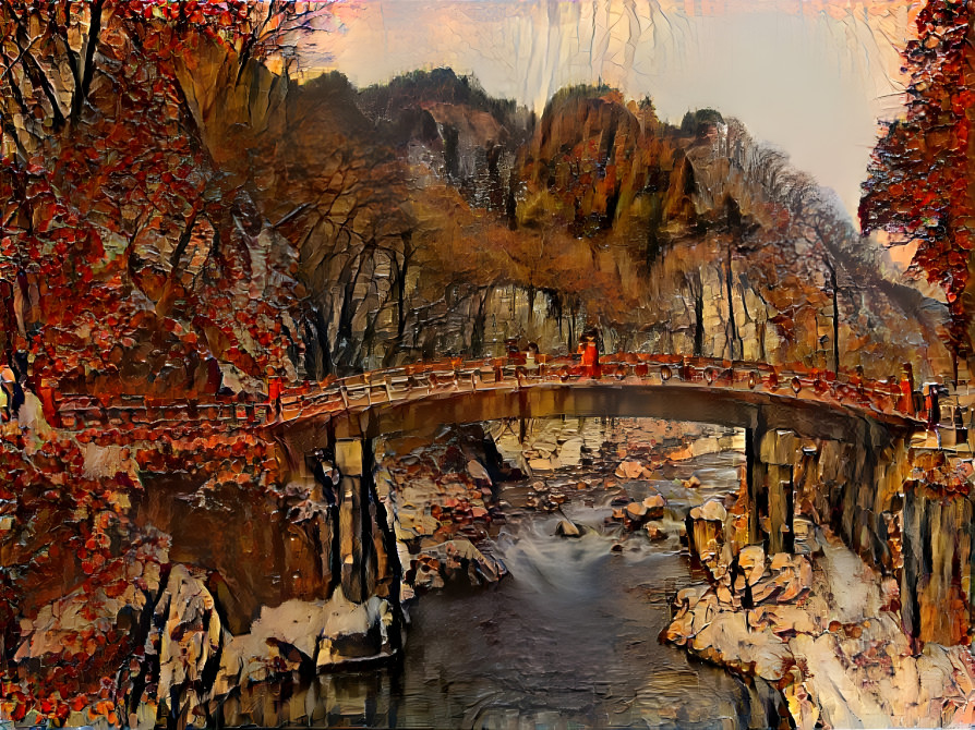
Style transfer applied to a picture of Shinkyo Bridge in Nikko (日光の神橋), using Google’s Deep Dream Generator

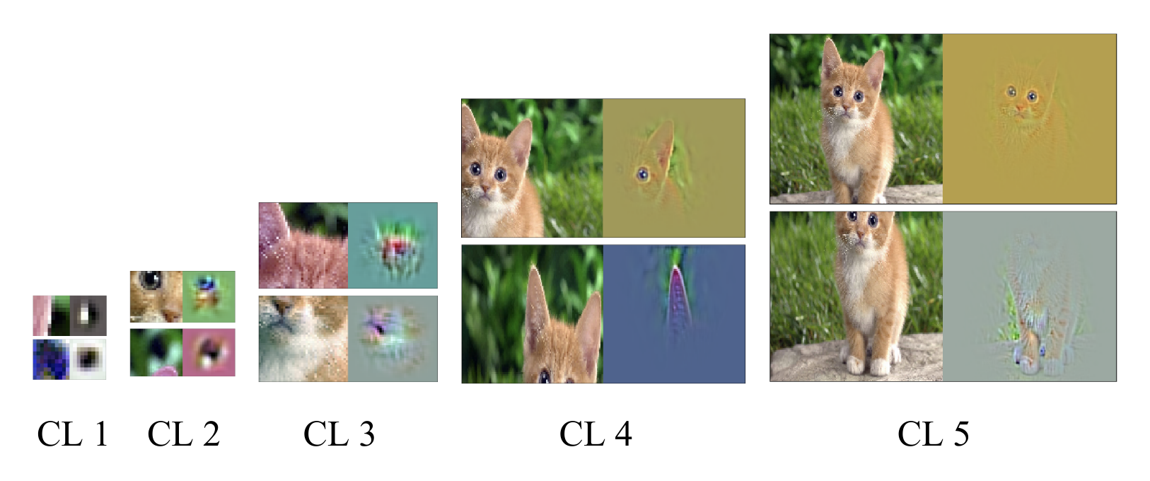
Convolutional networks find spatial relationships in multidimensional data (most often images), which allow computers to detect patterns to make predictions or modify the input images in surprising ways. The following image shows a series of feature map visualizations for a convolutional neural network, extracted from a picture of a cat: features related to the eyes, ears, or details as fine as pupil types.

For the style transfer example shown above, the original image is transformed so that it looks similar to a target style image until they’re virtually indistinguishable using the information from the filters:

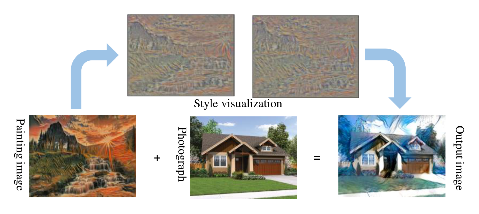
Convolution Visualization images from: Qin, Z., Yu, F., Liu, C., & Chen, X. (2018). How convolutional neural network see the world-A survey of convolutional neural network visualization methods. arXiv preprint arXiv:1804.11191.

Notebook Setup¶

Today we’ll be training CNNs, a process which can be very slow when run on a CPU. Instead, we’ll be relying on GPU processing! Thankfully, we can easily make the switch on Colab!

(If you’re running the notebooks on your own computer, you may have to jump through a few hoops in order to take advantage of your computer’s GPU)

Do note, however, that access to GPUs on Colab is somewhat limited - running your model’s training too many times may limit your access to the GPU resources at Google.

Changing the Runtime to GPU on Colab¶

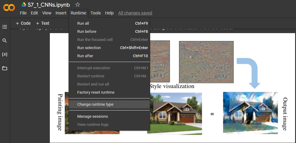
Click on the runtime dropdown menu and click on "change runtime type"

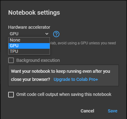
Then select "GPU" on the hardware accelerator dropdown menu

Once you’ve changed the runtime type, run the Notebook setup cell. A message confirming that you’ve succesfully changed runtime type should be printed 😃

In the setup cell, let’s import a few common modules, ensure MatplotLib plots figures inline and prepare a function to save the figures. We’ll also check that Python 3.9 or later is installed, as well as PyTorch ≥2.0 and TorchVision.

Data Setup¶

Today, we won’t be working on the MNIST dataset! Instead, we’ll be working on the tf_flowers dataset, and we’ll be attempting to train a Neural Network to learn to classify the flowers into 1 of 5 flower species: daisies, dandelions, roses, sunflowers, and tulips.

Let’s begin by loading the data. It’s about two-hundred megabytes, so — to keep this repository’s own dataset snapshot under its 50 MB-per-file limit — it’s committed here split into six smaller chunks that we’ll re-download and reassemble.

Q1) Load the flower_photos dataset. Split it into a training, validation, and test set (75% / 15% / 10%).¶

Hint 1: The cell above already reassembles the dataset into a directory of one subfolder per flower species (flowers_root) — exactly the layout torchvision.datasets.ImageFolder expects.

Hint 2: Once you have the full dataset as an ImageFolder, use torch.utils.data.random_split() to carve it into three Subsets. It takes a list of split sizes (as sample counts, or as fractions that sum to 1) — [0.75, 0.15, 0.10] gives you the split we want.

Hint 3: ImageFolder has a .classes attribute with the flower names, in the order used for the integer labels — you’ll want to keep a reference to it, since a Subset doesn’t expose it directly.

We now have a set of variables that have the training, validation, and test sets, as well as class_names. Let’s go ahead and define a function that will let us visualize our data.

Q2) Define a function that takes in a dataset, its name, and the list of class names, prints out how many samples are in the dataset, and displays a set of samples from the dataset.¶

Hint 1: len(dataset) gives you the number of samples in any PyTorch dataset (or Subset).

Hint 2: You can use the rnd_gen.integers() generator to pick a set of random indices into the dataset, then index the dataset with each one (dataset[index] returns an (image, label) pair). This is the same pattern as the sample_plotter function from the artificial-neural-networks exercises — you can reuse that approach here.

Hint 3: A dataset image tensor from ImageFolder has shape (channels, height, width), so before calling plt.imshow() you’ll need to move the channel dimension to the end with .permute(1, 2, 0).

And now let’s run the function on each of our training, validation, and test sets...

Q3) Run your defined visualization function on each of the training, validation, and test sets.¶

If everything worked out fine, you’ll have a grid of nicely labeled flower photos as your output:

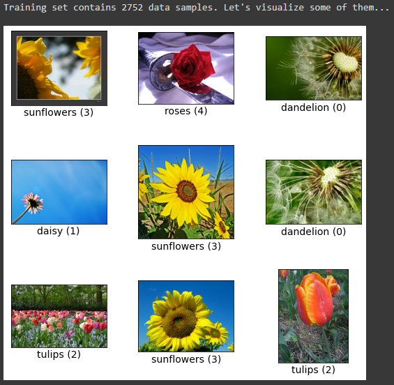
The flowers look very nice! (“And I’d be pretty bad at classifying them myself...” - a botanically challenged TA)

However, there is one sore point for our purposes - the images have different resolutions. Why is this a sore point? Well, in our architecture we’ll eventually flatten our convolutions and connect them to a dense layer, and as such we will need for all of the images to have the same dimensions! (There are other ways to address the issue of resolution, but we won’t discuss these for now)

We also note that our toTensor transform already scaled the pixel values to fall between 0 and 1 — one fewer thing to worry about compared to the raw 0–255 integers.

Let’s write a preprocessing transform that resizes every image to a common size!

Q4) Write a preprocessing transform that resizes images to 128x128.¶

Hint 1: torchvision.transforms.v2.Resize((height, width)) resizes an image tensor to a fixed size.

Hint 2: You can chain it onto the toTensor pipeline from Q1 using T.Compose([...]).

Q5) Recreate the dataset (and its train/validation/test split) using the new preprocessing transform.¶

Hint 1: random_split()'s three-way split isn’t affected by which transform the underlying dataset uses — as long as you re-create full_dataset with transform=preprocessing_transform and re-run random_split() with the same seed, you’ll get the same three subsets, just resized this time.

At this point I’d also like to point out that our dataset is not set up to be taken in batches. If you index a single sample, you’ll extract a single (image, label) pair — not a batch of them.

We actually want to work in 32 image batches, so let’s go ahead as set up data loaders for our datasets.

Q6) Wrap each of the training, validation, and test sets in a DataLoader with a batch size of 32.¶

Hint 1: You can define a batch_size variable to guarantee that the batch size is updated for all three loaders if you change the value and rerun this cell.

Hint 2: Only the training loader needs shuffle=True — we don’t need to shuffle validation or test data.

If we now take a sample batch like we did before, we’ll notice that there’s now a leading batch dimension in the shape!

Now that we’ve verified that our data loaders work as intended, let’s go ahead and build our model!

Model Setup and Training¶

Let’s begin by setting up everything we need to track our runs! This time, we want to work with multiple runs, and in order to visualize them independently in TensorBoard, each run needs to write to its own log directory.

Q7) Define a function that returns a filepath with the format './CNN_logs/run_CURRENT-DATE-AND-TIME'¶

Hint 1: Numpy includes a method to return the current date and time as a datetime64 object. Call the datetime64 method with 'now' as an argument on the numpy library, then convert it to a string.

Let’s try out our function! It should return something like: ./CNN_logs/run_2022-04-10T18:49

As in the artificial-neural-networks exercises, we’ll track training with a manual early-stopping counter, a checkpoint saved with torch.save() whenever the validation loss improves, and a SummaryWriter for TensorBoard.

Q8) Set up the early-stopping counter, best-validation-loss tracker, checkpoint filename, and TensorBoard writer for a CNN model without data augmentation.¶

Hint 1: See the artificial-neural-networks exercises for the pattern — a patience value, a best_val_loss initialized to infinity, an epochs_without_improvement counter, and a checkpoint filename to pass to torch.save().

We now have everything we need to track a training run. Let’s go ahead and define the model! Though let’s go ahead and clean up our random states first for consistency.

Q9) Define a convolutional neural network model. Do not use data augmentation techniques! We want to use this same architecture + data augmentation later, so we can compare the two.¶

Hint 1: There is at least one small, immediate change from the architecture below that will make its performance more effective — see if you can spot it once you’ve trained it.

Hint 2: nn.Conv2d needs an explicit number of input channels — the first convolution’s input has 3 (RGB), and every later layer’s input channels equal the previous layer’s output channels.

Hint 3: nn.LazyLinear infers its input size the first time data flows through it, so you don’t need to compute the flattened size by hand after four poolings — unlike nn.Linear, which requires it upfront.

Hint 4: As in the artificial-neural-networks exercises, leave the very last layer as a plain nn.LazyLinear/nn.Linear with no activation — nn.CrossEntropyLoss expects raw logits, not softmax probabilities.

Q10) Define the loss function, optimizer, and accuracy metric. We recommend nn.CrossEntropyLoss as the loss function, Adam as the optimizer, and torchmetrics.Accuracy for the metric.¶

Q11) Train the CNN model!¶

Hint 1: Write the same training-and-validation loop as in the artificial-neural-networks exercises: a training phase over train_loader, a validation phase over valid_loader inside with torch.no_grad():, TensorBoard logging with writer.add_scalar(), and checkpointing/early stopping based on patience.

Hint 2: This dataset is larger and the model deeper than in the MNIST exercises, so don’t be surprised if training takes a while — especially without a GPU.

Well, the performance of our CNN is likely underwhelming:

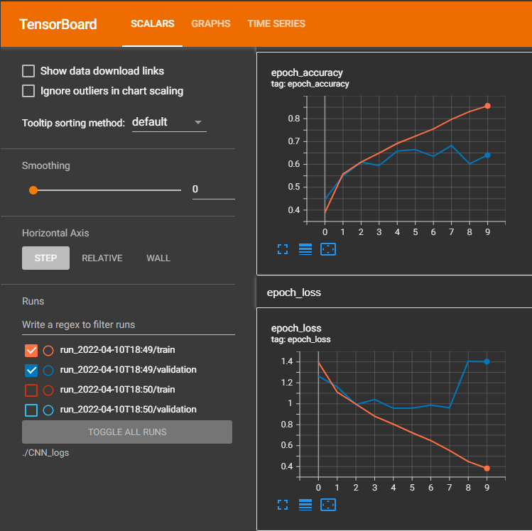
The model didn’t have too hard a time learning on the training set, but the validation loss quickly diverged and we started overfitting our training data. 😯

A common way to try to address this is by augmenting our training data - we can flip and rotate our images and it shouldn’t make too large a difference.

“A rose by any other name would smell as sweet” - Shakespeare

“An upside down rose is still a rose” - A significantly less talented poet than Shakespeare

Q12) Set up the early-stopping counter, best-validation-loss tracker, checkpoint filename, and TensorBoard writer for a CNN model with data augmentation.¶

Q13) Train an identical model to that defined in Q9, with the exception of RandomHorizontalFlip and RandomRotation augmentation transforms added to the training set’s preprocessing.¶

Hint 1: Unlike Keras, where RandomFlip/RandomRotation are layers inside the model, PyTorch applies data augmentation as part of the dataset’s transform — so this means building a second ImageFolder (with its own random_split, same seed) whose transform chains T.RandomHorizontalFlip() and T.RandomRotation(degrees) onto the Q5 preprocessing pipeline, then wrapping its training subset in a new DataLoader. The validation and test loaders should stay exactly as they were — we don’t want to augment the data we evaluate on!

Q14) Define the loss function, optimizer, and accuracy metric, exactly as in Q10.¶

If everything went according to plan, your model including data augmentation should perform a little better:

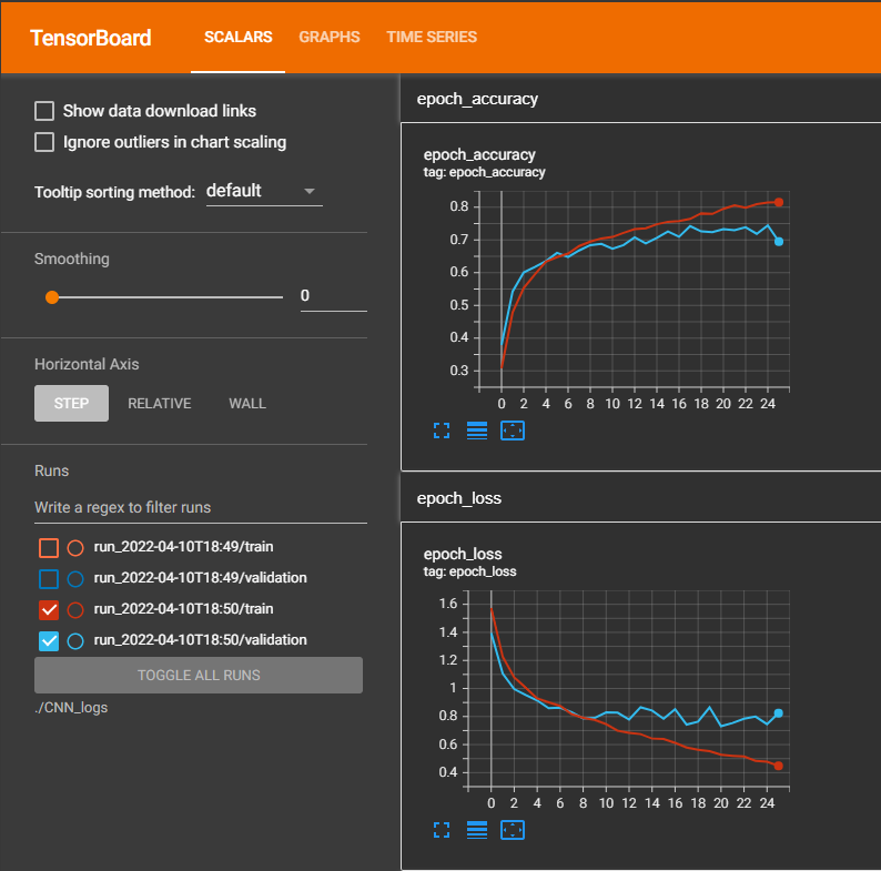
Now let’s run tensorboard and compare your two runs!

If everything went well, the model trained on the augmented data should have a lower accuracy on the training set compared to the original, but the better of the two should generalize better to unseen data — i.e. score a higher accuracy on the validation and test sets. Let’s check by reloading both models’ best checkpoints and evaluating them on the test set.