5.2) (Exercise) Artificial Neural Networks with PyTorch

This notebook was designed to be run on Google Colab and we recommend clicking on the Google Colab badge to proceed.

Photo Credits: Galaxy's Edge by Rod Long licensed under the Unsplash License

The defnition of AI is a highly contested concept. It often refers to technologies that demonstrate levels of independent intelligence from humans. By its very defnition, it is an intelligence that is differentiated from natural intelligence; it is a constructed, artificial, or machine intelligence.
$\quad$ Ryan, M. (2020). In AI we trust: ethics, artificial intelligence, and reliability. Science and Engineering Ethics, 26(5), 2749-2767.

This notebook, whose first draft was written by Milton Gomez, covers Chapters 9 and 10 of Géron’s “Hands-On Machine Learning with Scikit-Learn and PyTorch”, and builds on the notebooks made available on Github.

Notebook Setup¶

First, let’s import a few common modules, ensure MatplotLib plots figures inline and prepare a function to save the figures. We also check that Python 3.9 or later is installed, as well as PyTorch ≥2.0 and TorchVision.

import torch
import torch.nn as nn

# TorchVision, to download and load the MNIST dataset
import torchvision

# To track streaming metrics and log to TensorBoard
import torchmetrics
import torch.utils.tensorboard

# Common imports
import numpy as np
import os

# to make this notebook's output stable across runs
rnd_seed = 42
rnd_gen = np.random.default_rng(rnd_seed)

# To plot pretty figures
%matplotlib inline
import matplotlib as mpl
import matplotlib.pyplot as plt
mpl.rc('axes', labelsize=14)
mpl.rc('xtick', labelsize=12)
mpl.rc('ytick', labelsize=12)

# Where to save the figures
IMAGES_PATH = "_files"
os.makedirs(IMAGES_PATH, exist_ok=True)

def save_fig(fig_id, tight_layout=True, fig_extension="png", resolution=300):
    path = os.path.join(IMAGES_PATH, fig_id + "." + fig_extension)
    print("Saving figure", fig_id)
    if tight_layout:
        plt.tight_layout()
    plt.savefig(path, format=fig_extension, dpi=resolution)

# Initialize the run_index
run_index = None

# Loading Tensorboard
%load_ext tensorboard

Data Setup

Today, we’ll once again be working on the MNIST handwritten digit database - we’re becoming experts in typography! ✍

Let’s begin by loading the dataset using the TorchVision library.

Q1) Load the MNIST dataset using TorchVision. Divide it into a training, validation, and test dataset¶

Hint 1: Here is the documentation for the TorchVision implementation of the MNIST dataset.

Hint 2: torchvision.datasets.MNIST(root=..., train=..., download=True) returns a dataset object with two useful attributes: .data, a tensor of raw pixel values, and .targets, a tensor of labels. Calling .numpy() on either gives you back a plain numpy array, exactly like Keras’s mnist.load_data() used to.

Hint 3: The train argument selects the training set (True, 60 000 images) or the test set (False, 10 000 images) — there is no separate validation split built in, so you’ll need to carve one out of the training set yourself.

Hint 4: Since the full training dataset includes 60 000 samples, try using 50 000 samples as training data and 10 000 samples as validation data.

# Load the MNIST dataset
train_full_set = torchvision.___.___(root="datasets", train=True, download=___)
test_set = torchvision.datasets.MNIST(root="datasets", train=_____, download=True)

X_train_full, y_train_full = train_full_set.___.numpy(), train_full_set.___.numpy()
X_test, y_test = test_set.___.numpy(), test_set.___.numpy()

# Split the data
X_train =
X_valid =
_______ =
_______ =

What does our data look like? Let’s get an idea of the values and figure out what kind of preprocessing we should do before training our neural network.

Q2) Print the shape of the training, validation, and test sets. Then, print the maximum and minimum input values.¶

Hint 1: You loaded the data as numpy arrays. Thus, you can rely on the built-in methods for finding the shape and min/max values.

Hint 2: Click for the documentation on ndarray.max(), ndarray.min(), and ndarray.shape

#Write your code here

If you used the same train/validation split as we did, you should have 50k samples in the training set, 10k in the validation set, and 10k in the test set.

Since the data represents grayscale image values, data values should vary between 0 and 255; Normalize the data by dividing it by 255.

Q3) Normalize the input data for the training, validation, and testing sets¶

Hint 1: The datasets are stored as simple numpy arrays, so you can perform arithmetic operations on them!

X_train = _____ / 255
_____ =
_____ =

We now have the normalized training, validation, and testing data that we’ll use to train our neural network. Before moving on, it might be worth it to make a small visualiation of samples in our data to ensure that everything worked out correctly.

Q4) To visualize a sample image, write a function that:¶

1) Takes in an input dataset and its labels, a number of rows, and a number of columns

2) Prints out a random n_rows by n_columns sample of images with their labels

Hint 1: You can use the rnd_seed.integers() generator to generate a set of integers between 0 and the number of samples, with a size of (rows,columns). Here is some documentation that can help. It’s best practice to take in the random generator as an argument for your function.

Hint 2: You can use matplotlib’s fig, axes = plt.subplots() to make a grid of axes and call the imshow() method on each ax in order to plot the digit. It is recommended that you use the cmap='binary' argument in imshow to print the digits in black and white. Click on the links for the documentation to plt.sublopts(), plt.imshow(), and the colormaps (i.e., cmap values) available in matplotlib.

Hint 3: You can iterate using numpy ndenumerate() method, which will return the n-dimensional index of the array and the element located there. This will be useful when iterating through the indices you generated and plotting the corresponding digit and label

Hint 4: Code snippet, if you’re feeling stuck

def sample_plotter(X, y, n_rows, n_columns, rnd_gen):
    assert type(X) == type(np.empty(0))
    indices = rnd_gen.integers(0,X.shape[0], size=(n_rows, n_columns))

    fig, axes = plt.subplots(n_rows, n_columns, figsize=(8,6))

    for idx, element in np.ndenumerate(indices):
        axes[idx].imshow(X[element], cmap='binary')
        axes[idx].axis('off')
        axes[idx].title.set_text(y[element])
    return

def sample_plotter(___, ___, ___, ___):

    # Create a set of indices to access the sample images/labels

    # Create a figure with n_rows and n_columns

    # Plot each selected digit
    for in :


    return None

Now that our function is defined, let’s go ahead and print out a 4 row by 8 column sample from each dataset.

Q5) Grab a 4x8 sample of digits from each dataset and print out the image and labels¶

#Write your code here!

We’re now ready to start developing our neural network. The first thing that we want to do is figure out an appropriate learning rate for our model - after all, we want to choose one that converges to a solution and is the least computationally expensive possible.

Let’s start by writing a small helper that lets us change the learning rate after every iteration (i.e., after every batch of data) — since PyTorch has no callback system for a plain training loop, we’ll just call it ourselves. We will set up what is called an exponential learning rate (that is, the learning will increase by a factor of $k$ after each iteration). Expressed mathematically,

\begin{align} \eta_{\scriptsize{t}} = \eta_{\scriptsize{0}} \, \cdot \, k^{\scriptsize{t}} \end{align}

(1)

where $t$ is the current iteration.

As a reminder, an epoch is an iteration through the entire training dataset, while a batch is an iteration through a predefined subset of it. It’s important to make this distinction, as ML algorithms are often trained in batches when dealing with large datasets, and we normally do not want to change the learning rate in between batches during model training. However, we will do so during this evaluation phase in order to determine an adequate learning rate.

We will therefore write a helper that will do two things after the end of each batch:

Keep a track of the losses
2) Adjust the learning rate by multiplying it by a predefined factor

Q6) Set up an ExponentialLR class that, after each batch, logs the value of the loss function and learning rate, and then multiplies the learning rate by a factor of $k$ ¶

Hint 1: A PyTorch optimizer stores its learning rate in optimizer.param_groups[0]["lr"] — that’s both how you read it and how you set it (there is no separate backend to go through, unlike Keras).

Hint 2: The class will need to take in the optimizer and the $k$ factor during its initialization (here’s a quick overview on the init constructor method and self arguments in classes, with a focus on python). You will also need to save an empty list as an attribute for both the losses and the learning rates.

Hint 3: Give the class a step(loss) method that we’ll call ourselves at the end of every batch, once we have the batch’s loss value.

class _____:  # define the ExponentialLR class
    # Start
    def __init__(self, optimizer, factor):
        self.____ = ____ # set the optimizer
        self.____ = ____ # set the factor
        self.____ = ____ # initialize the losses list
        self.____ = ____ # initialize the learning rates list

    def step(self, loss):
        # Add the value of the learning rate to the list
        self.___.append(self.___.param_groups[0]["___"])

        # Add the value of the loss
        self.___.append(___)

        # Set the value of the learning rate and make it adjustable
        self.___.param_groups[0]["___"] *= self.___

Now that we’ve defined our helper, we can go ahead and start thinking about our neural network. For consistency’s sake, let’s start by setting our random state.

# Run this cell
torch.manual_seed(rnd_seed)

Let’s make a simple neural network model using PyTorch. For this, we will rely on nn.Sequential, since we will want all of the inputs of one layer to be fed into the next layer. We recommend using the architecture described in the diagram below, but feel free to define your own architecture!

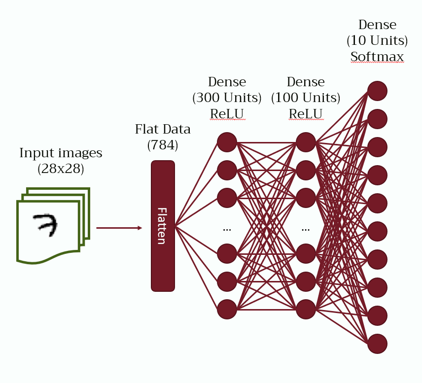
Q7) Write a sequential PyTorch model that will predict the digit class.¶

Hint 1: You can add the layers in the sequential model when initializing it. It expects the layers as separate arguments, e.g. nn.Sequential(layer1, layer2, ...). Check out the documentation here.

Hint 2: The input images should be flattened before feeding them into any densely connected layers. Here is the documentation for the flatten layer.

Hint 3: You want to use simple, densely connected layers for this exercise. Here is the documentation for the linear (densely connected) layer.

Hint 4: Unlike Keras, PyTorch’s nn.CrossEntropyLoss (which we’ll use to compile the model) expects raw scores (logits), not probabilities — so the output layer should NOT have a softmax activation. Leave the final layer as a plain nn.Linear, with the number of units set to the number of classes (e.g., the number of different digits in the MNIST dataset: 10).

# Create your model! Feel free to use our outline, or make your own from scratch

model = nn.___(  # call the sequential model class
                            ___,  # 1st Layer
                            ___,  # 2nd Layer
                            ___,  # 3rd Layer
                            ___) # 4th Layer

Now that we have a model defined, PyTorch has no single .compile() method like Keras — instead, we create the loss function, the optimizer, and the evaluation metric as separate objects:

The loss function will be set to cross entropy
2) The optimizer will be set to Stochastic Gradient Descent with a learning rate of 1e-3
3) We’ll track accuracy using the torchmetrics library

Q8) Define the loss function, optimizer, and accuracy metric with the given hyperparameters, and instantiate the helper we defined previously using a $k$ factor of 1.005 (i.e., a 0.5% increase in learning rate per batch)¶

Hint 1: Here is the documentation for the cross entropy loss function in PyTorch. It’s referenced as nn.CrossEntropyLoss().

Hint 2: Here is the documentation for the Stochastic Gradient Descent optimizer in PyTorch.

Hint 3: Here is the documentation for the accuracy metric implementation in the torchmetrics library. You’ll want torchmetrics.Accuracy(task="multiclass", num_classes=10).

___ = nn.___() # Set the loss function
___ = torch.optim.___(___.parameters(), lr=___) # Set the optimizer and learning rate
___ = torchmetrics.___(task="___", num_classes=___) # Set the accuracy metric

exponential_lr = _____(_____, factor=____)

PyTorch also has no built-in .fit() — training happens in an explicit loop over batches, supplied by a DataLoader. Let’s wrap our normalized training tensors accordingly before going any further.

# Run this cell
train_dataset = torch.utils.data.TensorDataset(
    torch.tensor(X_train, dtype=torch.float32),
    torch.tensor(y_train, dtype=torch.long))
train_loader = torch.utils.data.DataLoader(train_dataset, batch_size=32, shuffle=True)

Let’s go ahead and train the model for a single epoch.

Q9) Write the training loop for a single epoch, calling the exponential learning rate helper we defined earlier after every batch. Then, plot the Loss vs Learning rate.¶

Hint 1: For each batch, the loop needs to: zero the optimizer’s gradients, run the forward pass, compute the loss, call .backward() on the loss, then call .step() on the optimizer. Here is the documentation for .backward().

Hint 2: After computing the loss for a batch, call exponential_lr.step(loss.item()) to log it and update the learning rate. .item() converts a single-value tensor to a plain Python float.

Hint 3: After training, you can access the recorded losses and corresponding learning rates using the attributes we defined in Q6!

for X_batch, y_batch in train_loader:
    ___.___()  # zero the gradients
    y_pred = ___(___)  # forward pass
    loss = ___(___, ___)  # compute the loss
    ___.___()  # backward pass
    ___.___()  # update the weights
    exponential_lr.___(___.___())  # log and update the learning rate

# Plotting
fig, ax = plt.subplots()

ax.plot(___.___, # learning rates
        ___.___) # losses

# Define a tuple with (min_learning_rate, max_learn_rate)
x_limits = ( min(___.___), max(___.___) )

# Set the xscale to logarithmic
ax.set_xscale('log')

# Draw a horizontal line at the minimum loss value
ax.hlines(min(____.___), #Find the minimum loss value to draw a horizontal line
          *x_limits, # the star unpacks x_limits to the expected num of args
          'g')

# Set the limits for drawing the curves
ax.set_xlim(x_limits)
ax.set_ylim(0, ____) # use the initial loss as the top y boundary

# Display gridlines to see better
ax.grid(which='both')

ax.set_xlabel("Learning rate")
ax.set_ylabel("Loss")

If you used the architecture we defined above with the learning rate we defined above, you should produce a graph similar to this one:

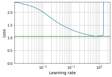
In this graph, you can see that the loss reaches a minimum at around 6e-1 and then begins to shoot up violently. Let’s avoid that by using half that value (e.g., 3e-1).

If you have a different curve, try setting your learning rate to half of the learning rate with the minimum loss! 😃

Now that we have an idea of what the learning rate should be, let’s go ahead and start from scratch once more.

# Run this cell - let's go back to a clean slate!
torch.manual_seed(rnd_seed)

We also want to instantiate the model again - the weights in our current model are quite bad and if we use it as is it won’t be able to learn since the weights are too far away from the solution. There are other ways to do this, but since our model is quite simple it’s worth it to just redefine it.

Q10) Redefine the model and its optimizer with the learning rate you found in Q9.¶

# redefine the model
model = nn.___( # call the sequential model class
    nn.___(), # flatten the data
    nn.___(), # densely connected ReLU layer, 300 units
    nn.___(), # densely connected ReLU layer, 100 units
    nn.___()) # densely connected layer, 10 units, no activation

___ = nn.___() # Set the loss function
___ = torch.optim.___(___.parameters(), lr=___) # Set the optimizer and learning rate

We’re now going to set up a saving directory in case you want to try running the model with different learning rates or other hyper-parameters!

#Change this number and rerun this cell whenever you want to change runs
run_index = 1

run_logdir = os.path.join(os.curdir, "my_mnist_logs", "run_{:03d}".format(run_index))

print(run_logdir)

We’ll also set up the tools to track training more carefully.

Early stopping. Instead of a callback, we’ll keep a simple counter that stops training if no improvement is found in the validation loss after a patience number of epochs.
2) Checkpointing. Instead of a callback, we’ll save the model’s weights with torch.save() whenever the validation loss improves, so we always keep the best version.
3) TensorBoard. PyTorch writes TensorBoard-compatible logs directly, via torch.utils.tensorboard.SummaryWriter. Handy 🙌!

writer = torch.utils.tensorboard.SummaryWriter(run_logdir)
patience = 20
best_val_loss = float("inf")
epochs_without_improvement = 0

Let’s go ahead and fit the model again!

Q11) Write the training loop for 100 epochs, with early stopping, checkpointing, and TensorBoard logging.¶

Hint 1: Wrap the validation set in a DataLoader too, the same way we did for the training set.

Hint 2: Each epoch has two phases: a training phase (as in Q9, but without the exponential learning rate helper this time) and a validation phase, where you run the model on the validation set inside a with torch.no_grad(): block (no gradients needed since we’re not training) and compute the average validation loss and the accuracy metric.

Hint 3: After computing the validation loss for an epoch, compare it to best_val_loss. If it’s lower, save the improvement (best_val_loss = ...), reset epochs_without_improvement to 0, and save the model with torch.save(model.state_dict(), "my_mnist_model.pt"). Otherwise, increment epochs_without_improvement, and break out of the loop once it reaches patience.

Hint 4: Log the validation loss and accuracy for the epoch with writer.add_scalar("name", value, epoch), once per metric.

valid_dataset = torch.utils.data.TensorDataset(
    torch.tensor(X_valid, dtype=torch.float32),
    torch.tensor(y_valid, dtype=torch.long))
valid_loader = torch.utils.data.DataLoader(valid_dataset, batch_size=___)

for epoch in range(___): # number of epochs
    # Training phase
    for X_batch, y_batch in ___:
        ___.___()
        y_pred = ___(___)
        loss = ___(___, ___)
        ___.___()
        ___.___()

    # Validation phase
    val_losses = []
    with torch.___():
        for X_batch, y_batch in ___:
            y_pred = ___(___)
            val_losses.append(___(___, ___).item())
            ___.update(___, ___) # update the accuracy metric

    val_loss = np.mean(___)
    val_accuracy = ___.compute().item()
    ___.reset() # reset the metric for the next epoch

    # TensorBoard logging
    writer.add_scalar("___", val_loss, ___)
    writer.add_scalar("___", val_accuracy, ___)

    # Checkpointing and early stopping
    if val_loss < ___:
        ___ = val_loss
        epochs_without_improvement = ___
        torch.save(___.___(), "my_mnist_model.pt")
    else:
        epochs_without_improvement += ___
        if epochs_without_improvement >= ___:
            break

Finally, we need to evaluate the performance of our model. Go ahead and try it out on the test set!

Q12) Evaluate the model on the test set.¶

Hint 1: Load the best saved weights back with model.load_state_dict(torch.load(...)), then switch the model to evaluation mode with .eval().

Hint 2: Reuse the same with torch.no_grad(): + metric.update() pattern from the validation phase in Q11, this time over a DataLoader wrapping the test set.

# Rollback to best model, which was saved during training
___.load_state_dict(torch.load("___", weights_only=True))
model.___() # switch to evaluation mode

test_dataset = torch.utils.data.TensorDataset(
    torch.tensor(X_test, dtype=torch.float32),
    torch.tensor(y_test, dtype=torch.long))
test_loader = torch.utils.data.DataLoader(test_dataset, batch_size=32)

with torch.___():
    for X_batch, y_batch in ___:
        y_pred = ___(___)
        ___.update(___, ___)

print(f"Test accuracy: {___.compute().item():.4f}")

Finally, we can use tensorboard to check out our model’s performance! Note that the tensorboard extension was loaded in the notebook setup cell.

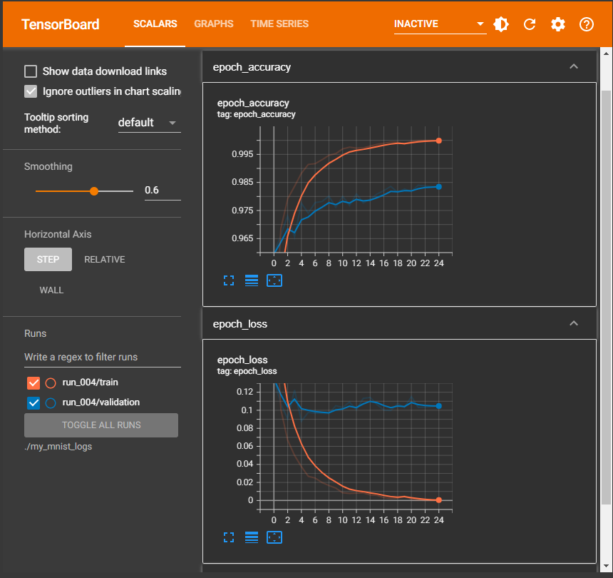
%tensorboard --logdir=./my_mnist_logs --port=6006

An enthusiastic (albeit somewhat sick 😷) TA noted that during the development of the notebook the accuracy reached on the test dataset was 97.84%. Additionally, the tensorboard curves from the test run is given below: